Network Flow Optimization by Genetic Algorithm and Load Flow Analysis by Newton Raphson Method in
Power System
By
Fahmid Iftekher Ali
(201116020)Md Monjurul Alam Rizvi
(201116031)Md Razuan Hossain
(201116047)Supervisor
Dr M Shamim Kaiser
A thesis submitted to Department of Electrical, Electronic and Communication Engineering, Military Institute of Science and Technology, Mirpur Cantonment, Dhaka in partial fulfillment of the requirements for the degree of Bachelor in Electrical, Electronic and Communication Engineering
Department of Electrical, Electronic and Communication Engineering Military Institute of Science and Technology,
Mirpur Cantonment, Dhaka, Bangladesh December 2014
Certification
The thesis titled, ―Network Flow Optimization by Genetic Algorithm and Load Flow Analysis by Newton Raphson Method in Power System‖, submitted by Fahmid Iftekher Ali, Monjurul Alam Rizvi and Razuan Hossain to the, has been accepted as satisfactory for the and approved to its style and contents.
Supervisor
Dr. M. Shamim Kaiser
Assistant Professor
Institute of Information Technology, Jahangirnagar University,
Savar, Dhaka-1342
Declaration
It is hereby declared that except for the contents where specific references have been made to the work of other, the studies contained in this thesis are the result of investigation carried out by the students under the supervision of Dr M Shamim Kaiser, Assistant Professor, Institute of Information Technology, Jahangirnagar University No part of this thesis has been submitted to any other university or other educational establishments for a degree, diploma or other qualifications (except for publication).
Signature of the Students
Fahmid Iftekher Ali Student ID – 201116020
Md Monjurul Alam Rizvi Student ID – 201116031
Md Razuan Hossain Student ID - 201116047
Acknowledgement
This thesis is the accumulation of our work on the Optimal Power Flow problem of Power system in the past one year. In this adventurous ride to our first ever step to scientific research we were greatly assisted by some very supportive and extremely sagacious persons in respective fields. We are using this opportunity to express our gratitude to everyone who supported us through the course of time.
First and Foremost, we have to thank our thesis supervisor, Dr. M. Shamim Kaiser, Assistant Professor, Institute of Information Technology, Jahangirnagar University.
Without his kind assistance and dedicated involvement in every step throughout the process, this paper would have never been accomplished. We would like to thank you very much for your help and understanding over the past year.
In the same fashion, we are lucky to have Capt M Mahbubur Rahman (BN) and Gp Capt Dr Hossam-E-Haider as the Dean, Faculty of Electrical and Computer Science,MIST and Head of the Department, Department of EECE, respectively.
Getting through the dissertation required more than academic support. We cannot begin to express our gratitude and appreciation to Mostafa Kamal Tareq, Hasib Ahmed Majumdar, Oyickotan-E-Dilshad, Nurul Islam Shihab, who have been unwavering in their personal and technical support during the time. We are thankful to everyone above as well as Maj Saleh Ahmed (BA), Capt Shueb Al Hasan (BA), SLt Manzurul Alam (BN) and SLt Nur Mohammad (BN) for their invaluably constructive criticism and friendly advice regarding the thesis work. We are sincerely grateful to them for sharing their truthful and illuminating views on a number of issues related to the thesis.
Last but not the least; we are indebted to our families for their continuous support through the ups and downs. Words fall short to express our deep sense of gratitude for their sincere encouragement and inspiration throughout the academic and non- academic life. We owe everything to them and without their assistance we could not have come this far let alone completed this thesis work. This dissertation stands as a testament to your unconditional love and encouragement.
Abstract
The optimal power flow within a system network is a pronounced problem now a day.
Basically power cannot be generated without considering the cost. Thereby it is always necessary to keep a relation between the generation of power and the total system cost.
Here our objective is to simulate an objective function to get the optimum power flow within the optimizing cost and also make a load flow analysis of the system.
There are a lot of techniques of optimization such as Classical optimization technique, Advanced Optimization Techniques, Simulated annealing Techniques, Interior Point (IP) method, Artificial Neural Network (ANN), Fuzzy Logic (FL) method, Genetic Algorithm method etc. Also there are several methods of load flow analysis for example Fast Decoupled Method,Newton Raphson Method, Bisection Method, Secant Method, False Position method etc. Among of them we have chosen Genetic Algorithm method for optimization and Newton Raphson Method for the load flow analysis.
By the approach of genetic algorithm we tried to find out per unit cost and the total cost of the 9 bus system. And here we also have taken an approach to find out the load flow analysis by simulation of a program where we have shown generation, injection in the buses and also the system losses etc. Both the methodological techniques were simulated in the MATLAB.
Contents
Chapter 1: Introduction ... 1
1.1 Background... 1
1.2 Assumptions and Limitation: ... 4
1.3 Objectives: ... 5
1.4 Outline of the paper ... 6
Chapter 2: Literature Review ... 7
2.1 General Discussion ... 7
2.2. Optimal power flow analysis: ... 8
2.2.1 Classical Optimization Techniques ... 9
2.2.2 Numerical Methods of Optimization ... 9
2.2.3 Advanced Optimization Techniques ... 10
2.2.4 Simulated annealing Techniques ... 10
2.2.5 Quadratic Programming (QP) method ... 10
2.2.6 Nonlinear Programming (NLP) method ... 10
2.2.7 Interior Point (IP) method ... 10
2.2.8 Artificial Intelligence (AI) methods ... 11
2.2.9. Why we use GA for cost optimization?? ... 14
2.3. Load flow analysis: ... 15
2.3.1 Historical background of power flow analysis: ... 16
2.3.2 Gauss-Seidel method ... 16
2.3.3 Newton Raphson Method ... 17
2.3.4 Fast Decoupled Method ... 17
2.3.5 Bisection Method ... 17
2.3.6 Secant Method ... 17
2.3.7 False Position method ... 18
2.3.8 Why we used Newton Raphson method?? ... 18
Chapter 3: Methodology ... 19
3.1 Genetic Algorithms in Optical Power Flow ... 19
3.2 Roulette wheel selection ... 27
3.3 Load Flow analysis... 28
Chapter 4: System Model and Problem Formulation ... 35
4.1 Model Power system ... 35
4.2 Problem Formulation ... 36
Chapter 5: Result and Discussion ... 38
5.1. Resolution Factor ... 38
5.2 Individual fitness value ... 39
5.3 Creating path sequence and summing per unit cost: ... 42
5.4 Total Cost of the system and maximum power in the buses: ... 44
5.5 Probability Calculation (Roulette Wheel Method) ... 45
5.6 Load Flow analysis by Newton-Raphson method ... 47
Chapter 6 : Conclusion ... 51
References ... 53
Appendix A : MATLAB program codes ... 55
A. Individual Fitness Calculation ... 55
B. Total System Cost by genetic algorithm: ... 56
C. Probability by Roulette Wheel Selection ... 58
D. Load Flow Analysis by Newton Raphson method ... 60
List of figures
Figure 1 : Cycle of reproduction of GA ... 21
Figure 2: Reproduction Cycle ... 22
Figure 3 Chromosome Modification ... 22
Figure 4: Evolution Process ... 24
Figure 5: Deletion Process ... 25
Figure 6 : A Simple flow chart of the GAOPF ... 26
Figure 7: Roulette Wheel Selection... 28
Figure 8: 3-Machines, 9-bus System ... 35
Figure 9: Individual Fitness Scenario of Bus 1 ... 41
Figure 10: Individual Fitness Scenario Bus 2 ... 41
Figure 11: Individual Fitness Scenario Bus-3 ... 41
Figure 12: Cost of Total System ... 44
Figure 13: Probability of Being Outcome (Bus-1) ... 46
Figure 14 Probability of Being Outcome (Bus-2) ... 46
Figure 15 Probability of Being Outcome (Bus-1) ... 47
List of Tables
Table 1: Parameter Set of Pgi ... 38
Table 2: Coding of Pgi parameter set ... 39
Table 3: Best Individual Fitness of the First Generator Bus ... 40
Table 4: Best individual fitness of the second Generator Bus ... 40
Table 5: Best individual fitness of the Third Generator Bus ... 40
Table 6: Probability of being the outcome ... 45
Table 7: Load Flow Analysis ... 49
Table 8: Line Flow & Losses ... 50
Chapter 1
Introduction
1.1 Background
Optimal Power Flows (OPF) has been useful in planning and real-time operation of power systems. OPF helps to minimize generation costs and system losses and helps in improvement of voltage profiles. Typically, there are two problems that have been assumed decoupled and these have been treated independently. However, as the system try to operate nearer to its stability limits, i.e. its voltage collapse point, because of market pressure, this assumption cannot be applied any longer and therefore needed to consider these limits applying OPF. For the improvement of the overall system security, optimization procedures can also be used by introducing these stability limits in the OPF problem.
The voltage stability problem is widely studied in power systems and the basic reasons that cause a network voltage collapse have been identified. [1]. It has been found that for a voltage collapse condition, the overall system stability is closely connected to the proximity of the system. if the system approaches to the voltage collapse point, the stability region becomes smaller in size, which results in a system having less capability of surviving possibilities .[2] Therefore, for first approximation, voltage stability criteria can be useful to account for the overall stability of the system. This adds that to study the voltage stability problem, optimization techniques can be useful. [3][4]
If we look from the market point of view, we would observe that over the course of the past two decades, there have been significant changes in electrical power industries.
Deregulated electricity markets which was first introduced in Chile in 1990, are now common place. These competitive markets are capable of reducing costs, but they also
enable uncertainty to generation forecasting as there is competition to sell electricity among the power producer. Meanwhile, in many places, consumer demand has outperformed infrastructure development by creating pressure on aging equipment.
Moreover, the complexity to the scheduling of power flows increased to another degree by the increased penetration of non-dispatch able renewable sources. All these factors enable contribution to the increasing need for fast and reliable methods of optimization.
Since the introduction by Carpentier (1962). [5] OPF has been the main method for such analysis. Since then Optimization methods are widely used in power system planning, operation, and analysis.
OPF tries to optimize a given cost by controlling power flow within an electrical network in such a way that it does not violate constraints of network power flow. OPF determines current, voltage and power that is injected throughout an electrical power system like conventional power flow analysis. However, there are some difference between OPF and conventional power flow. OPF works with an under constrained system where capable of producing multiple solutions.
Classical optimization methods are often used to solve OPF. Usually the OPF has been considered as the minimization of an objective function which represents the generation cost as well as the loss during transmission. The physical laws governing the power generation-transmission system and the equipment‘s operating limitations are considered as constraints.
The general OPF problem is considered as large-scale optimization problem which may include both continuous and discrete control variables. The constraints under consideration and address of particular objective function decide in which name the resulting optimization problems can be termed. Irrespective of the name, a set of power flow equations in the constraints is included by optimization problem of any power system can be classified as a form of OPF. Over the years there has been huge
development of many OPF solution methods, each of these have distinct mathematical characteristics and computational requirements. However, OPF problems in real life are often significantly more difficult than that of the problems we consider classically and on
the basis of requirement of solution of different engineering application and adaptibility to the modeling, OPF methods vary significantly. Therefore, till now , all the various forms fo OPF problems do not have single formulation and solution.
With the increase of network size and complexity, the difficulty of solving OPF also increases.
Recent industry developments have significantly increased complexity of electric power system, forwarding this issue to the further OPF research. Typically utilities had relatively few generators in prior decades compared to the numbers of generators introduced today. The reason is the introduction of independent power producers and integration of distributed and renewable generation in large-scale. Meanwhile, variables to the load side of OPF problems are added by demand response programs.
Because of the advancement of the OPF solution techniques, effective optimal power flow is limited by
the power system‘s high dimensionality
The incompleteness of domain dependent knowledge of power system engineers.
The first limitation can be solved by numeric optimization procedures based on
successive linearization. The successive linearization can be solved using the first and the second derivatives of the objective functions and their constraints.
Genetic algorithms (GAs) introduce a new and powerful solution to optimization problems. The increase of availability of high performance computers at relatively low costs has made it possible. These algorithms are widely used in solving global optimization searching problems when the technique of closed-form optimization is not applicable.[6] Genetic algorithms are considered as parallel and global search techniques that are capable of emulating natural genetic operators. The GA is more likely to converge toward the global solution because it calculates many points in the parameter space simultaneously. It is not needed to assume whether the search space is differentiable or continuous. [7] In recent papers [8], the Genetic Algorithm Optimal
Power Flow (GAOPF) problem is solved based on the use of a genetic algorithm load flow. To accelerate the concepts it suggests the use of gradient information by the use of the steepest decent method. The method is not sensitive to the starting points.
Moreover, within the constraints range and objective functions, it is capable of determining the global optimum solution to the OPF. But GAOPF has a requirement and that is two load flow should perform per individual, per iteration because the fitness includes all controllable variables. In this paper we develop a simple genetic algorithm applied to the problem of optimal power flow in large power distribution systems. To accelerate the processes of GAOPF, the controllable variables are decomposed to active constraints. These affect the cost function directly that is included in the process of Genetic algorithm. Conventional load flow program helps to update passive constraints, only, one time after the convergence on the GAOPF. To take the effect of the passive constraints, the slack bus parameter would be recalculated in the load flow process.
1.2 Assumptions and Limitation:
The advantages of such methods are in their mathematical underpinnings, but as the problem formulation and algorithm selection are sensitive, the disadvantages arise.
The reliable use of expert systems is precluded by Incompleteness of domain knowledge where rule completeness in not possible.
Here we have just considered only 9 bus system but in IEEE bus bar topology there exists 14 bus system,30 bus system,57 bus system which is not considered in our procedure.
In the power system grid power flow controller are also used such as unified power flow controller (UPFC), thyristor switched capacitor (TSC), thyristor controlled series capacitor (TCSC), thyristor controlled rectifier (TCR) etc are used but in our thesis we didn‘t consider those power flow controller.
Protective equipment‘s such as circuit breaker , relay, trip circuit are not used in this system
In the load flow analysis we have used slack bus and PQ bus generator but we don‘t consider the PV bus in the system generator.
Here we can‘t done the load flow analysis by genetic algorithm if we can did it then it will be a best scheme to make an comparison between GA an Newton Raphson load flow analysis.
1.3 Objectives:
The main objectives of this work are to minimize the cost of the power system and to maximize the power flow. The other objectives are
To enhance the power flow in transmission lines and
To keep the power outputs of generators, bus voltages, shunt capacitors/reactors and transformers tap-setting in their secure limits.
To study the per unit cost and the total network cost of the 9 bus system
To simulate a program for the load flow analysis
To optimize the system cost and within the cost maximizing system load flow
1.4 Outline of the paper Chapter 1
Chapter 1 deals with the introduction of the paper and this part consists of background history , problem statement , assumption and limitation , objectives, outline of the paper ,methodology of our working process where genetic algorithm , newton raphson load flow analysis, roulette wheel selection etc process are described.
Chapter 2
In the chapter 2 literature review section takes place where we have described about the optimal power flow technique and also load flow analysis technique. Further we have described here about the reason of using Genetic Algorithm and Newton raphson method.
Chapter 3
Chapter 3 describes the system which we have considered has described and the formulation of the problem has done.
Chapter 4
Chapter 4 is designed with the result portion and the calculation procedure. Resolution factor , individual fitness, summing up the per unit cost and the total cost of the system, probability calculation, load flow analysis etc. are the part of this section. Here we have also discuss of the each section of the results.
Chapter 5
Chapter 5 deals with the conclusion of our thesis and the scope of further future works in this section. Further references which we have used here are provided in this chapter.
Chapter 2
Literature Review
2.1 General Discussion
Optimization technique has been used to minimize the cost or the object through the objective function considering equality and inequality constraints.
Engineering applications of optimization technique are:
Scheme of an aircraft within an optimum level of weight
Defining the optimal routes of the space vehicle
Planning out civil engineering work such as bridge, building, chimney , towers for reducing the cost
Scaling out a suitable structure for the earthquake, wind and other random loading.
Designing plastic optimal infrastructure
Minimizing product cost in case of selection of machine condition while metal cutting process
Idol design of machine tools, gears and other mechanical components
Optimal design of chemical processing plants and equipment
Scheme of pump , turbine, heat transferring equipment for the maximization of power flow in the system
Record in controlling
Monitoring the idle and waiting time of the production line to reduce the cost of the production
Develop a best strategy to maximize the profit for the plant
Progression of the optimization model depends over five phases, such as:
Data collecting
Defining problem and then formulate it
Development of the model
Validation of model and then evaluate its performance
Application of model and interpreting it criteria
2.2. Optimal power flow analysis:
The main aim of Optimal Power flow (OPF) algorithm is to capture a steady state operating point. Generation cost, loss are curtailed by steady state operating point.
Further, it also maximizes load ability preserving a suitable system representation in terms of parameters of generators (real and reactive powers, line flow limits, output of various compensating devices etc.). Usually, classical optimization methods were used but as the technology have advanced and integration of FACTS devices in the power system, the traditional concepts and practices of power systems are placed over by an economic market management. . Therefore, OPF has become complex in nature. So, Artificial Intelligence (AI) methods are used which can solve higher complexity problem than OPF. [11]
Some optimization methods are described in the following section:
2.2.1 Classical Optimization Techniques
This method helps to find out unconstrained maxima or minima of continuous and differentiable functions. Classical optimization techniques can solve three types of problem whose are:
1. multivariable functions with no constraints, 2. Single variable functions,
3. Multivariable functions with both equality and inequality constraints.
2.2.2 Numerical Methods of Optimization
Numerical methods of optimization consist of the following section:
1. Linear programming: provide an event where the objective function f is linear and set A which is considered as design variable space is specified using only linear equalities and inequalities. (A is the design variable space)
2. Integer programming: considers linear programs where selected or all variables are constrained to proceed with integer values.
3. Quadratic programming: where set value A is specified with linear equalities and inequalities allowing the objective function in quadratic terms.
4. Nonlinear programming: studies on the objective function or the constraints or both the nonlinear sections.
5. Stochastic programming: where some of the constraints depend on random variables.
6. Dynamic programming: where the optimization strategy comprised of splitting problem into smaller sub problems.
7. Combinatorial optimization: which is concerned with problems where the set of feasible solutions is discrete or can be reduced to a discrete one.
8. Infinite-dimensional optimization: where the set of feasible solutions is a subset of an infinite-dimensional space, such as a space of functions.
9. Constraint satisfaction: studies the case in which the objective function f is constant (this is used in artificial intelligence, particularly in automated reasoning).
2.2.3 Advanced Optimization Techniques
Hill climbing: It is a graph search algorithm technique where the current path is extended with a successor node which is closer to the solution than the end of the current path. Basically, Hill climbing is used widely in artificial intelligence fields.
2.2.4 Simulated annealing Techniques
the main aim of Simulated annealing Techniques is to bring the system from an arbitrary initial state to a state having the minimum possible energy where each point of the search space is compared to a state of some physical system, and the function is considered as the internal energy of the system within the state.
2.2.5 Quadratic Programming (QP) method
Among the mathematical optimizing problem Quadratic programming (QP) is a distinctive method of Optimizing problem. The main objective of QP is to optimize (minimize or maximize) a quadratic function of different variables whose are subjected to the linear constraints of those variables.
2.2.6 Nonlinear Programming (NLP) method
Nonlinear programming (NLP) deals with problems involving nonlinear objective and constraint functions. NLP is a mathematical process of solving optimization problem where a system is considered with both equality and inequality constraints.
2.2.7 Interior Point (IP) method
Interior point methods are a particular type of algorithm which can solve both linear and nonlinear convex optimization related problems. Convex minimization, which is considered as a sub field of optimization deals with minimizing convex function over convex sets. IP method is also known as barrier method.
2.2.8 Artificial Intelligence (AI) methods
Artificial Intelligence (AI) is considered as a science or a technique to develop intelligent computer program. It consists of three type of method whose are
1. Artificial Neural Network (ANN) 2. Fuzzy Logic (FL) METHOD 3. Genetic Algorithm (GA) METHOD ARTIFICIAL NEURAL NETWORK (ANN)
Artificial Neural Network (ANN) is considered as information processing criteria that are enlightened by the method of biological nervous system (such as the brain) to process information. Generally ANN system composed of large number of interconnected elements (in terms of biology which is called neurons) to solve specific problems. In biological system, whole synaptic system exists in between the neurons which is also true in case of ANN system. Application of ANN system is pattern reorganization, data classification.
FUZZY LOGIC (FL) METHOD
Fuzzy Logic (FL) introduces a logic which is more than simple true or false values.
Declaration is made with the degrees of truthfulness and falsehood by the fuzzy logic. It is a sort of many valued logic. It proposes the reason rather than the fixed or exact thing of an incident. FL variables have special type of true value whose degree ranges from 0 to 1,. that means such type of true is considered as partial true which is in the range of completely true or completely false. An example corresponding to FL is given that , if today is sunny could be 100 % true if there is no cloud in the sky , but 80 % true if few cloud exists, again 50% true if its hazy , further 0 % true if there is rain all day long.
GENETIC ALGORITHM (GA) METHOD
Genetic Algorithm method is a technique of optimization. It was pioneered by John Holland in 60s and after then GA is widely used, experimented and applied different engineering fields. To use GA one must represent a solution to the problem as a chromosome. Thereby GA generates a population of solution and involves mutation, cross over operator on it to develop a solution in order to the best one for the system.
There are three basic outlines which should be performed to operate the GA technique, whose are
Describe of the objective function.
Implementation of the genetic representation.
Introduction to the genetic operators.
Now, let‘s go through an example to understand GA clearly,
First we have shown genome encoding of three chromosomes in a discrete value abcd ( chromosome 1) s1 sz (chromosome 2) n1 (chromosome 3)
To evaluate the new generation, the mutation operator provides random changes on few individual to go through the outside of local optima. Here we have used bit flip mutation.
Bit flip mutation is considered with two step process.
Algorithm generates a random binary vector, selects individual genes for the mutation where the vector is denoted by 1.
Then the algorithm swaps each selected gene with a new selected gene randomly through the data base
Individual:
abcd s1 sz n1
Random Vector:
0000 1 0 1
Child:
abcd S1 sz N1
The main application of GA is
To optimize system cost
To maximize network power flow
To optimize and planning for Travelling salesman problem
To learn the behavior of the robot through GA
To localize an objective is a complex scene , etc
Further progression after genetic algorithm:
A. MISCELLANEOUS AI METHODS
These approaches are used to specify the programmable characteristics of AI through multiple states. Generally AI technique doesn‘t need this thing.
B. EVOLUTIONARY PROGRAMMING (EP)
There are four major evolutionary algorithm paradigms and Evolutionary programming is one of them. It is quite similar to the genetic programming but the main difference is the structure of the program which is optimized is fixed while its numerical parameters are allowed to develop.
C. ANT COLONY OPTIMIZATION (ACO)
Ant colony optimization (ACO) which is also known as probabilistic technique where computational problems are reduced to find out a good path and graphical method is used to find out the optimize path for the system. A set of software known as artificial
ant search is used to find out the optimization problem in the field of ACO. To apply the ACO method, the optimization problem is converted into the best path on a weighted graph and the artificial ant software build a solution by moving through the graph incrementally.
D. PARTICLE SWARM OPTIMIZATION (PSO)
Particle swarm optimization (PSO) in a computational method where an iterative process takes place to optimize the problem and fetch out a candidate solution for a given measure quality.
PSO was pioneered by Kennedy, Eberhart and Shi and they intended it for simulating social behavior. PSO optimizes a problem taking a population candidate solutions which are consider as dubbed particles. Then providing this particle around search space in accordance with the simple mathematical formulae terminated over the particles position and velocity.
2.2.9. Why we use GA for cost optimization??
OPF has been basically considered to minimize an objective function containing generation cost or transmission loss. Normally classical methods are used to solve the OPF problems. But there are operating limitations in the classical method of optimization. And the limitations are
High dimension and complex interconnection of the power system.
Power system engineers having an incomplete domain dependent knowledge.
The first limitation which can solved by numerical optimization procedures which is based on the successive linearization where we use first and second derivatives of objective function as well as their constraints. The advantage of GA is that it is mathematical supporting techniques but also having some disadvantage like sensitivity of problem formulation and algorithm selection also exists.
The second limitation for incomplete domain knowledge GA offers a new and powerful approach to solve optimization problems by increasing the availability of high performance computer within relatively low cost
Basically GA technique is parallel and global search technique that deals with the natural genetic operators. GA is more likely to global solution and at the same time it assesses many points in the parameter space. Genetic algorithm optimal power flow (GAOPF) is evaluated based on the usage of the GA load flow. GA method is not sensitive in the starting point of analysis and proficient to determining the global optimum solution of OPF through an objective function. We can improve a simple GA technique to solve large power distribution system.
2.3. Load flow analysis:
Load/power flow analysis determines the flow of the real and reactive power and their ratings in a network. As far as the power system is a multifunction and interconnected system. Load flow analysis is complex in nature. Generally is load flow study single line diagram, per unit measurements are considered. By the by a line data , resistance , reactance , load demand, magnitude and phase angle of voltage, generation ,injection, real and real power etc. are also subjected in the load flow analysis. It studies the power flow in the system both the steady state condition and on duty cycle condition.
Load flow analysis is an important part and parcel for the future planning as well as obtaining the best operation of the existing system. Load flow analysis calculates voltage drop in each bus bar and power flow in all branches and the feeder circuit. We can determine the faulty condition on the network with the load flow analysis. This analysis also gives us the idea to distribute power through the feeder. Losses in each branch and the total system power losses are also calculated through the load flow analysis. Essential planning, economic scheduling, and control of existing system etc.
strategies are taken through the load flow analysis.
2.3.1 Historical background of power flow analysis:
Improvement in electrical power system was first recognized over half a century ago resulting in benefit over interconnected system power transport. But at that time it was critical to predict the voltage and flows in the network component. As day by day network has been developed, the challenge has undertaken to deal with the consisting network. Power flow analysis is a tool for the engineer to provide a status on generator and load system.
In the earlier decades load flow analysis are done by the calculation board. This board is such a type of analog computer board and there was emulated specific system using physical lumped parameter inductor, capacitor, and resistor to realize the actual system and also these components are connected in the same topology. To study the flow a team of engineers were worked together to adjust the setting and reading out the result and thereby there is a need to find an alternative solution for the load flow analysis.
In the earliest decades load flow analysis are done by the Gauss-Seidel method which made possible to solve the load flow problem for relatively large system for the first time. But due to having poor convergence characteristics Newton Raphson(NR) algorithm technique was developed to improve the Gauss Seidel technique. Then the problem arises over NR method is that to solute a matrix over large dimension.
Following the advances and the extension development in the load flow analysis in the
‗60s upcoming in the earlier of the ‗70s there comes fast decoupled load flow whose computational technique is higher than the previous ones
Some methods of load flow analysis are given below:
2.3.2 Gauss-Seidel method
This method is considered for the load flow analysis and also known as the method of successive displacement or the Liebmann method. It is an iterative method to solve the linear system equation. It provides slower rates of convergence with compared to other iterative methods. But the main advantage is it needs a little memory and does not need to solve the matrix in the system.
2.3.3 Newton Raphson Method
Newton Raphson(NR) method fetches an iterative process to approach one root of a function. This method begins with the initial estimation of all unidentified variables (voltage magnitude, angle at load buses and voltage angle at generator buses). Then a Taylor series is introduced and higher terms are ignored. This thing is done for each of the power balance equations included in the system.
2.3.4 Fast Decoupled Method
Also known as ―fixed slope, decoupled NR‖ that exhibits a variation of NR model and inexact decoupling of active and reactive flows in the system in addition it fixes the value of jacobian matrix. The main properties of this method are:
Practical power transmission having high X/R ration through the grid.
Real power changes are less sensitive to the voltage magnitude changes.
Reactive power changes are less sensitive to the angle of the voltage magnitude.
2.3.5 Bisection Method
Bisection method approaches root finding criteria that repeatedly bisects an interval and choose the subinterval in which a root supposed to be lied. It is very simple and robust process. This method is also known as binary search method as well as interval halving method.
2.3.6 Secant Method
In the mathematical analysis of a system Secant method is the algorithm to find out the roots in the secant lines to provide a better approximation of a root of a function. The secant method is considered as a finite difference approximation of NP method. The secant method holds only the most recent estimation therefore the root does not necessarily required to be bracketed.
2.3.7 False Position method
The false position method is the problem solving method where arithmetic, algebra, and calculus techniques are used .the beginning of this method is to determine the problem using test values which is named as false value and then adjust the value in accordance with the preference. The features of Bisection Method and Secant Method both are combined in the false position method.
2.3.8 Why we used Newton Raphson method??
One of the fastest methods for meeting the root.
Meets on the root quadratic ally.
It‘s easy to renovate to multiple dimensions.
The roots which are found from other methods used to be polished by this method.
Easy to solute the nonlinear equation where higher order are ignored. [12]
.
Chapter 3
Methodology
3.1 Genetic Algorithms in Optical Power Flow
A. Description of Genetic Algorithms
Evolutionary algorithms have another branch which is genetic algorithms. They all are computational models which are inspired in the nature. Based on the mechanism of natural selection and natural genetics the genetic algorithms are powerful stochastic search algorithms. Works lay down by GA with a population of binary string by searching many peaks paralleled. They exchange information between the peaks by employing genetic operators. It also reduces the possibility of ending at a local optimum.
No search methods are flexible enough like GAs as because the other search methods requires information about the quality of the solution produced by each parameter set(
objective function values) and not take different optimization methods those shows the requirement of derivative information and may be it worsen complete knowledge of the problem structure and parameters.[9]
Differences between GAs and general searching algorithms are:
1. Opposing to a single point and searching many peaks in parallel the algorithms work with a population of string.
2. Strings of characters represent the parameters set but not the parameters themselves are worked under GAs.
3. Deterministic rules are not used by GA but probabilistic transition.
4. Instead of derivatives or others auxiliary knowledge GAs use objective function information.
5. Simultaneously GAs has the potential to find solutions in many different areas.
B. Components of a GA
The process by which a problem is solved using GAs follows:
the encoding technique (gene, chromosome),
Initialization procedure (creation),
Evaluation function (environment),
Selection of parents (reproduction),
use of Genetic operators (mutation, recombination)
Parameter settings (practice and art).
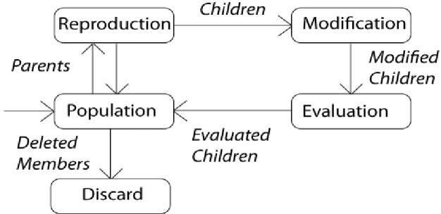
Thus the components can be summarized as: population, reproduction, modification, evolution and deletion. [10]
C. Simple Genetic Algorithm {
Initialize population;
Evaluate population;
While Termination Criteria Not Satisfied {
Select parents for reproduction;
Perform recombination and mutation;
Evaluate population;
} }
Figure 1 : Cycle of reproduction of GA D. Description of the procedure
D.1. Population
Chromosomes could be:
Bit strings (0101 ... 1100)
Real numbers (43.2 -33.1 ... 0.0 89.2)
Permutations of element (E11 E3 E7 ... E1 E15)
Lists of rules (R1 R2 R3 ... R22 R23)
Program elements (genetic programming)
... any data structure ...
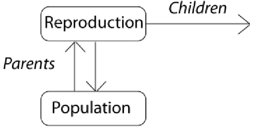
D.2. Reproduction
Parents are selected at random with selection chances biased in relation to chromosome evaluations.
Figure 2: Reproduction Cycle D.3. Chromosome Modification
Chromosome Modifications are stochastically triggered. Two operators are widely used in chromosome modification.
Operator types are:
Mutation
Crossover (recombination)
Figure 3 Chromosome Modification
Crossover: Recombination
Crossover is the primary genetic operator. It promotes the exploration of new regions in the search space. The recombination operation divides two strings into segments by setting a crossover point at random for a pair of parents which is selected from the population, i.e. Single Point Crossover. The segments from the parents behind the
crossover point are exchanged with each other so that these can generate their offspring.
P1 (0 1 1 0 1 0 0 0) (0 1 0 0 1 0 0 0) C1 P2 (1 1 0 1 1 0 1 0) (1 1 1 1 1 0 1 0) C2
The crossover operator greatly accelerates search early in evolution of a population. It introduces the opportunity of effective combination of schemata (sub solutions on different chromosomes)
Mutation: Local Modification
Mutation is a secondary operator .It prevents the early conclusion of the algorithm in a local solution. The definition of mutation operator can be stated as a random segment change in a particular string with a low probability of such change. It is Mutation which adds a random search character to the genetic algorithm, and it is important to avoid that, after some generations, all possible solutions were very similar to each other.
Before: (1 0 1 1 0 1 1 0) After: (0 1 1 0 0 1 1 0)
Before: (1.38 -69.4 326.44 0.1) After: (1.38 -67.5 326.44 0.1)
D.4 Evaluation
In the evolution process, it decodes a chromosome and assigns it in a fitness measure.
The evaluator is considered as the only link between a classical GA and the problem it is solving
Figure 4: Evolution Process D.5. Deletion
Deletion performs by removing a duplication gene from the chromosome and when the deletion occurs the effective mutation rate gets decreased.
There are two types of deletion, such as
Deletion and duplication
- In this process two bits are randomly selected and then their previous bits are duplicated
Example: before duplication 00 1001 0 Deletion 00 10- - 0 Duplication 00 1010 0
Deletion and regeneration
- In this process bits in the cross site are deleted and at the same time generated randomly.
Example: before regeneration 10 0110 1 Deletion 10 - - - - 1 Regeneration 10 1101 1
Figure 5: Deletion Process
E. GA applied to OPF
E.1. Chromosome coding and decoding
Gas deals with the binary string population. With the binary coding method, the active generation power set 9-bus test system would be coded as binary string of 0‘s and 1‘s with different lengths. The choice of the bit-string length is concerned with the resolution. The resolution is specified by the designer in the search space.
E.2. Crossover
For a pair of parents, the bit string segments before the random cross over point are exchanged to create two offspring. The new strings can be considered as the next generation of possible solutions. The selection of the strings to be crossed is done according to their scores. The scores are determined by using the roulette wheel.
E.3. mutation
A single bit operator is used by the mutation operator. From a chosen string, generally a random bit value changes. It provides an added search characters in the search space.
E.4. reproduction:
Reproduction process is based on the principle of survival of the better fitness.
According to their fitness value, the operator obtains a fixed number of copies of solutions. The increment of no of copies is dependent on the score. A score value is connected to a particular solution according to its distance of the optimal solution (closer distances to the optimal solution mean higher scores).
E.5. Fit of candidate solutions and cost function The cost function is defined as:
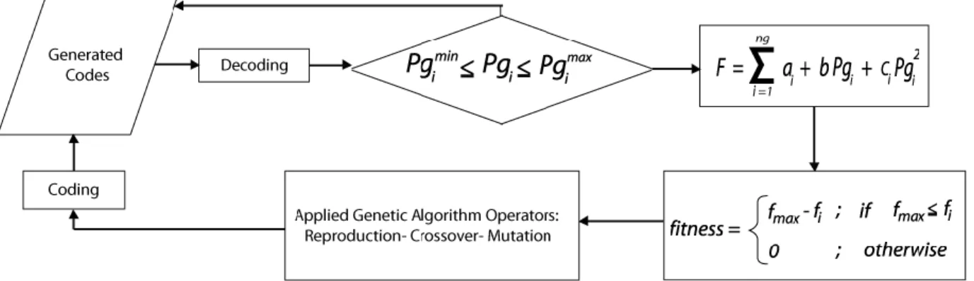
Our objective is to search (Pg1, Pg2, and Pg3) in their allowable limits to achieve the optimization problem of OPF. The cost function F(x) choses a chromosome (a possible (Pg1, Pg2, Pg3) and returns a value. The value of the cost is then mapped into a fitness value Fit (Pg1, Pg2,Pg3) so that it can fit in the genetic algorithm.
Minimizing F(x) is equivalent to achieving a maximum fitness value in the searching process. A chromosome having lower cost function should be assigned a larger fitness value. The objective of OPF has to be changed to the maximization of fitness to be used in the simulated roulette wheel as follows:
Then the GA tries to generate better offspring for the improvement of the fitness.
A standard GA procedure for solving the optimal power flow problem is summarized in the diagram of the Figure 6.
Figure 6 : A Simple flow chart of the GAOPF
3.2 Roulette wheel selection A. General Description
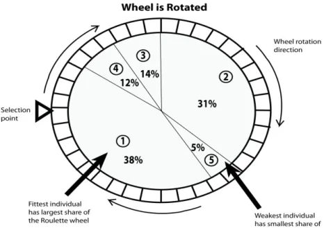
Roulette wheel selection is a genetic operator. It is used in genetic algorithms for choosing possible useful solutions for recombination. In fitness proportionate selection, like all other methods of selection, fitness is assigned by the fitness junction to possible solutions or chromosomes. If fi is the fitness of individual i is the population, its probability of being selected is pi=fi / ΣNj=1fj, where N is the number of individuals in the population.
This could be assumed similar to a Roulette wheel in a casino. Usually on the basis of fitness value, a part of the wheel is assigned to each of the probable selections. This could be achieved by dividing the fitness of a selection by the total fitness of all the selections, thereby normalizing them to 1. Then on the basis of procedure of rotation of roulette wheel, random selection can be made.
Though there is less chance of elimination of candidate solution of higher fitness, still there is small possibility that they may face it. If we consider a less sophisticated selection algorithm, such as truncation selection, it will eliminate a fixed percentage of the candidates which are weak in nature. With fitness proportionate selection there is a possibility that some weaker solutions may survive the selection process. This is an advantage because a solution may be weak but it may add some components which could prove useful following the recombination process.
B. Selection of the fittest
The basic part of the selection process is to stochastically select from one generation to create the basis of the next generation. The fittest individuals have a greater chance of survival than weaker ones is the main requirement. This has a clear indication that fitter individuals will tend to have a better probability of survival and will go forward to form the mating pool for the next generation. There is a chance for weaker individuals too. In nature such individuals may have genetic coding that may prove useful to future generations.
Figure 7: Roulette Wheel Selection
3.3 Load Flow analysis
To apply the newton-Raphson method to the solution of the power fow equation, bus voltages and line admittances are expressed in polar form. For ith bus in the system, the real and reactive power equations are:
(1) (2)
When , the corresponding terms are separated from the summation,
These equations can be readily differentiated with respect ot voltage angles and magnitudes. The terms involving and are obtained from the definition of and the fact that the angle is zero when
The power mismatches for a typical load bus are,
(3) (4)
In order to describe the procedure in a simpler way, a four bus system is taken as example. And from now on, equations are based on this assumption.
For a real power ,
The last three terms can be multiplied and divided by their respective voltage magnitudes without altering their values,
A similar mismatch equation can be written for reactive power ,
Each non slack bus of the system has two equation like those for and . Collecting all the mismatch equations in to vector –matrix form yields,
(5)
The mismatches for the slack bus and are undefined when and are not scheduled. The terms and are also omitted because those corrections are both zero at the slack bus.
The solution of equation (5) is found by iteration as follows:
Estimation of the values and for the state variables.
Using the estimates to calculated from equations (1) and (2), mismatches equation (3) and (4), and the partial derivative elements of Jocobian
Finding solution of equation (5) for the initial corrections and .
Addition of the solved corrections to the initial estimates to obtain,
Using new values of and as starting values for iteration 2 and continue.
In more general terms, the update formulas for the starting values of the state variables are,
For the four bus system sub matrix has the form
Expressions fo the elements of this equation are easily found by differentiating the appropriate number of terms in equation (1). When the variable equals the particular value , only one of the cosine terms in the summation of equation (1) contains , and by partial differentiating that single term with respect to the typical off-diagonal elements of ,
On the other hand, every term in the summation of equation (1) contains and so the typical diagonal element of is,
By comparing this expression and that for in equation (2),
In a quite similar manner, we can derive formulas for the elements of sub matrix as follows:
(6)
(7) Comparing this equation for with equation (1) for , it can be showed,
(8)
The elements of sub matrix are easily found by first finding the expression for the derivative and them multiplying by to obtain
Comparison with equation (6) yields
This is a most useful result, for it reduces the computation involved in forming the jacobian since the off-diagonal elements of are now simply the negatives of the corresponding elements in . This fact would not have become apparent if we had not multiplied by the magnitude . In an analogous manner, the diagonal elements of are found to be
And comparing this result with equations (7) and (8),
Finally the off-diagonal and diagonal elements of sub matrix of the Jacobian are determined to be
Now bringing together the results developed above in the following definitions:
Off-diagonal elements,
Diagonal elements,
Interrelationship amon the elements in the four sub matrices of the jacobian are more clearly seen if we use the definitions to rewrite equation (5) in the following form:
Chapter 4
System Model and Problem Formulation
4.1 Model Power system
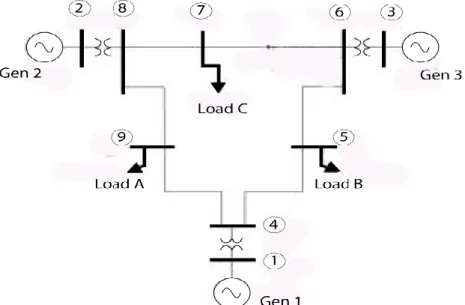
The GAOPF has been developed by MATLAB programming. The system considered is a IEEE 3 machines, 9 bus system. This IEEE 9 Bus Test Case represents a portion of the Western System Coordinating Council (WSCC) 3-Machines 9-Bus system.
Basically, this 9 bus system contains 3 generators, 9 buses and 3 loads.
The base KV levels in the go from 16.5 kV to 230 kV. The line complex powers are around hundreds of MVA each. As a test case, this one has few voltage control devices and is easy to control.
Figure 8: 3-Machines, 9-bus System
4.2 Problem Formulation
The standard OPF problem can be written in the following form, Minimize F(x) (the objective function)
Subject to:
hi(x) = 0, i = 1, 2, ..., n (equality constraints) gj(x) = 0, j = 1, 2, ...,m (inequality constraints)
Where x is the vector of the control variables that is those which can be varied by a control center operator (generated active and reactive powers, generation bus voltage magnitudes, transformers taps etc.)
The most commonly used objective in the OPF problem formulation is the minimization of the total cost of real power generation. The individual costs of each generating unit are assumed to be function, only of active power generation and represented by quadratic equation of second order. The objective function for the entire system then be written as the sum of the quadratic cost model at each generator.
Where ng is the number of generation including the slack bus. Pgi is the generated active power at bus i. ai, bi and ci are the unit costs curve for ith generator.
While minimizing the cost function, its necessary to make sure that the generation still supplies the load demands plus losses in transmission lines. Usually the power flow equations are used as equality constraints.
Where the active and reactive power injection at bus I are defined in the following equation
The inequality constraints on the problem variables considered include:
• Upper and lower bounds on the active generations at generator buses
• Upper and lower bounds on the reactive power generations at generator buses and reactive power injection at buses with VAR compensation
• Upper and lower bounds on the voltage magnitude at the all buses
• Upper and lower bounds on the bus voltage phase angles:
It can be seen that the generalized objective function F in non-linear and the number of equality and inequality constraints increase with the size of the power distribution systems. Applications of a conventional optimization technique such as the gradient- based algorithms to large power distribution system with a very non-linear objective functions and great number of constraints are not good enough to solve this problem.
Because it depends on the existence of the first and the second derivatives of the objectives of the objective function. [13]
Chapter 5
Result and Discussion
5.1. Resolution Factor
The Genetic Algorithm works with a population of binary string, not the parameters themselves. For simplicity and convenience, binary coding is used in this paper. With the binary coding method, the active generation power set of the 9-bus system ( Pg1, Pg2, Pg3) would be coded as binary string of 0‘s and 1‘s with length B1, B2, B3
respectively. in this process, in order to determine the power level in each generation bus, a resolution factor is used. The resolution factor Ri can be defined as:
Where, Ui is the lower bound of parameter Pgi Li is the upper bound of parameter Pgi Bi is the bit length of the binary coding
The parameter domain of the ( Pg1, Pg2, Pg3) is presented in the Table 1 Table 1: Parameter Set of Pgi
Bus Type Pmin Pmax a b c
1 slack bus .6 2.1 110 2.5 .01
2 PV bus .15 2.4 120 3 .05
3 PV bus .2 .95 100 4 .25
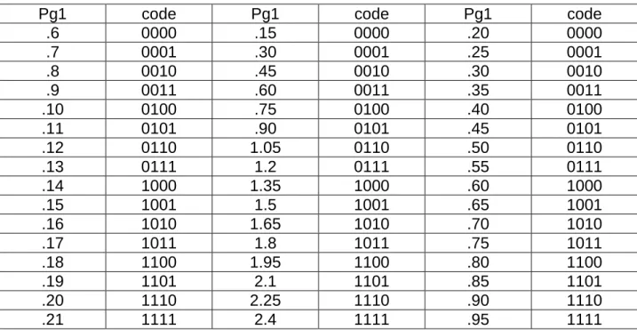
Considering the resolution factors for (Pg1, Pg2, Pg3) be (.1, .05,1) we have (B1, B2, B3) = (4, 4, 4).
The total number of power levels in each bus is 16. The parameter set can be coded according to the following Table 2. The power levels of the generator bus 1 are in a range of 0.6 to .21 per unit value. Accordingly, the range of generator bus 2 and generator bus 3 are .15 to 2.4 and .20 to .95 respectively.
Table 2: Coding of Pgi parameter set
Pg1 code Pg1 code Pg1 code
.6 0000 .15 0000 .20 0000
.7 0001 .30 0001 .25 0001
.8 0010 .45 0010 .30 0010
.9 0011 .60 0011 .35 0011
.10 0100 .75 0100 .40 0100
.11 0101 .90 0101 .45 0101
.12 0110 1.05 0110 .50 0110
.13 0111 1.2 0111 .55 0111
.14 1000 1.35 1000 .60 1000
.15 1001 1.5 1001 .65 1001
.16 1010 1.65 1010 .70 1010
.17 1011 1.8 1011 .75 1011
.18 1100 1.95 1100 .80 1100
.19 1101 2.1 1101 .85 1101
.20 1110 2.25 1110 .90 1110
.21 1111 2.4 1111 .95 1111
5.2 Individual fitness value
Our goal is to search the (Pg1, Pg2, Pg3) in their admissible limits to achieve the optimization problem of OPF. The cost function F(x) takes a chromosome (a possible Pg1, Pg2, Pg3) and returns a value. The value of the cost is then mapped into a fitness value Fit (Pg1, Pg2, Pg3) so as to fit the genetic algorithm.
As mentioned above, the general cost function F(x) is taken
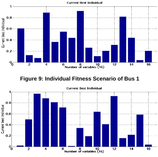
In this process, the best 3 of the individual fitness value has been chosen through a MATLAB using the cost function. In case of the ―Gen 1‖, the top three fitness values are found at the power level 1.3, .6 and .14 pu. The result of the simulation is as follows in Table 3
Accordingly, the best three individual fitness of the generator 2 are shown in the Table 4. The best individual fitness is found at the power level .45, 2.1 and 1.8 and coded as 0010, 1101, and 1011 respectively.
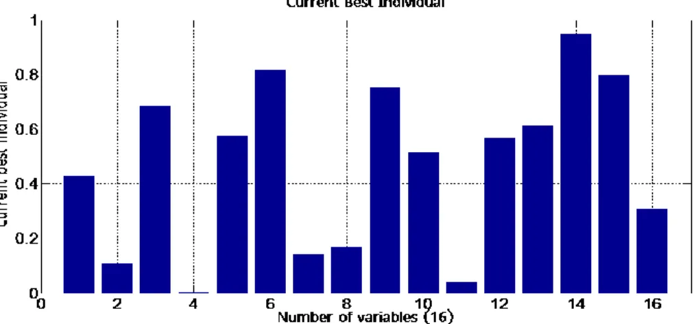
For generator 3, the top individual fitness value were at .85, .95 and .45.The parameters of Generator 3 in shown in the Table 5
Table 3: Best Individual Fitness of the First Generator Bus
Ranking Individual fitness Rmks
1. .85 Pg1=.13 code = 0111
2. .82 Pg1=.6 , code = 0000
3. .75 Pg1=.14 code = 1000
Table 4: Best individual fitness of the second Generator Bus
Ranking Individual fitness Rmks
1. .88
P
g2=.45 code = 0010
2. .82
P
g2=2.10
code =1101
3. .81
P
g2=1.8
code =1011
Table 5: Best individual fitness of the Third Generator Bus
Ranking Individual fitness Rmks
1. .9
P
g2=.85 code = 1101
2. .88
P
g2=.95 code = 1111
3. .85
P
g2=.45 code = 0101
The simulation result is shown in a graphical manner below:
Figure 9: Individual Fitness Scenario of Bus 1
Figure 10: Individual Fitness Scenario Bus 2
Figure 11: Individual Fitness Scenario Bus-3
5.3 Creating path sequence and summing per unit cost:
The power flow from a source bus to a destination bus will be most economical through the fittest path. Thereby, the cost of transmission of power will be optimized by this path. The most fit path will be the combination of the fittest segment of the from bus to bus of the power system.
The total system transmission cost will be the summation of the individual cost of power transmission from the three buses towards the next destination. the individual power transmission cost for each bus can be calculated from the general non-linear cost function.
To calculate the optimum cost of transmission the fittest path for first, second and third generation bus are taken into consideration
For Generator 1, the per unit voltage level P
gi= .13, and the values of constants a, b, c associated with bus are 110, 2.5 and .01.
Thus,
For Generator 2, the per unit voltage level P
gi= .45, and the values of constants a, b, c associated with bus are 120, 3 and .05.
Thus,
For Generator 2, the per unit voltage level P
gi= .85, and the values of constants a, b, c associated with bus are 100, 4 and .25.
Thus,
Thereby, the cost through this path is the sum of F1, F2, F3.
=
Corresponding chromosome bit of the path: 011100101101
Following the same procedure again for the second fittest paths for each generation bus,
Corresponding chromosome bit for the path: 000011011111
for the third fittest paths for each generation bus,
Corresponding chromosome bit for the path: 100010110101
So, the path that consists of the top fittest path segments has the lowest
transmission cost. Therefore, the Optimum path will comprise of the fittest path
segments.
5.4 Total Cost of the system and maximum power in the buses:
Genetic Algorithm uses the process of iteration to find out the cost of the total power system. The MATLAB program code of Genetic Algorithm has been collected from the Website of Math works incorporation. To calculate the total cost of power transmission a data matrix was given input to the program. The data matrix consists of the constants a, b, c along with the minimum and maximum power of the bus. The input data matrix is,
The population size was set to 12 as the binary representation of the each path from source to destination is a combination of 12 bits (i.e. 110011001011). The ‗generation‘
means the number of iteration. It is set to 100 for this thesis paper. The higher the number of iteration, the higher will be the accuracy in the result. And, the total load demand is assumed as 240MW.
The optimum power transmission cost of the system was found 3631624.980. But the mean cost is a way higher than the best value. It is shown as 375857.2354. And within this cost, the generator 1 can serve up to 95 MW, generator 2 up to 115 MW and the third generator can 75 MW.
Figure 12: Cost of Total System