trend analysis with twitter hashtags by monjur bin shams id

(1)

TREND ANALYSIS WITH TWITTER HASHTAGS

BY

MONJUR BIN SHAMS ID: 161-15-6812

AND

MD. JUNAED HOSSAIN ID: 131-15-2187

This Report Presented in Partial Fulfillment of the Requirements for the Degree of Bachelor of Science in Computer Science and Engineering

Supervised By

Dr. Sheak Rashid Haider Noori

Associate Professor and Associate Head Department of CSE

Daffodil International University

DAFFODIL INTERNATIONAL UNIVERSITY

DHAKA, BANGLADESH DECEMBER 2019

(2)

i

©Daffodil International University

(3)

ii

(4)

iii

ACKNOWLEDGMENT

First, we express our heartiest thanks and gratefulness to Almighty God for His divine blessing makes us possible to complete the final year project/internship successfully.

We really grateful and wish our profound our indebtedness to Dr. Sheak Rashed Haider Noori, Associate Professor & Associate Head, Department of CSE Daffodil International University, Dhaka. Deep Knowledge & keen interest of our supervisor in the field of “Data Mining & Machine Learning” to carry out this project. His endless patience, scholarly guidance, continual encouragement, constant and energetic supervision, constructive criticism, valuable advice, reading many inferior drafts and correcting them at all stages have made it possible to complete this project.

We would like to express our heartiest gratitude to Dr. Syed Akhter Hossain, Professor and Head, Department of CSE, for his kind help to finish our project and also to other faculty members and the staff of CSE department of Daffodil International University.

We would like to thank our entire coursemates at Daffodil International University, who took part in this discussion while completing the course work.

Finally, we must acknowledge with due respect the constant support and patience of our parents.

(5)

iv

ABSTRACT

Social media has converged into our everyday life in such a way that from lifestyle to our behaviors, we follow the social media immensely. The influence of social media is easily observable whenever any ‘TREND’ occurs in social media platforms and we stumble over the internet to follow that. Detecting trends can help to get notified about not only the ongoing topics around the internet as well as it gives us the chance to understand people’s choices, emotions and so on. This study of trend analysis becomes more specific and invaluable when it is targeted for a specific genre or community. As such- Gaming, Movies

& Tv series viewers, etc. There are very few assets in twitter for those specific genres which could assist its audiences or consumers to keep track of the trend list of that particular genre. Our chosen genre was Gaming. The primary purpose of our research is to analyze and predict the ongoing trends around Twitter of this specific community using Twitter Hashtags, which is a short yet quite stronger mode of expressing one’s mood or the gist of any topic. Our contribution to the research reflects in applying the LSTM model of Recurrent Neural Network model in a time series dataset which was unconventional and more complex than the existing methods of analyzing regular time series models.

(6)

v

CHAPTER 3: RESEARCH METHODOLOGY

^08-24

3.1 Introduction 08-09

3.2 Research Subject and Instrumentation 09-13

3.3 Data Collection Procedure 13

3.3.1 Time Series Dataset Nature 13-18

3.4 Statistical Analysis 19-20

3.5 Implementation Requirements 21

3.5.1 Data Normalization: Min-Max Scaler 21

3.5.2 Batch Function 22

3.5.3 RNN LSTM Model with TensorFlow 22

3.5.4 The Constants of the LSTM Model 22-23

3.5.5 Loss Function & Optimizer 23-24

CHAPTER 4: Experimental Results & Discussion

^25-27

4.1 Experimental Results 25-26

4.2 Descriptive Analysis 26-27

4.3 Summary 27

CHAPTER 5: Summary, Conclusion, Recommendation and Implication for Future Research

28-31

5.1 Summary of the Study 28

5.1.1 Trends in Business 28-30

5.1.2 Trends in Technology 30

(8)

vii

5.2 Conclusion 30

5.3 Recommendations 31

5.4 Implications to Further Study 31

APPENDIX A

³²

REFERENCES

^33-34

PLAGIARISM REPORT

³⁵

(9)

viii

LIST OF FIGURES

FIGURES PAGE NO

Figure 3.1.1: Trend list of Twitter on April 3, 2019 08

Figure 3.2.1: Workflow of an RNN model[18] 12

Figure 3.3.1.1: A dataset where only trend is present[11] 14 Figure 3.3.1.2: A dataset where only seasonality is present[12] 14 Figure 3.3.1.3: A dataset where trend and seasonality both are

present[13]

15

Figure 3.3.1.4: Hashtag count on April 3, 2019 16

Figure 3.3.1.5.: Hashtag count of game names on October 29th, 2019 17 Figure 3.3.1.6: Graphical representation of the hashtag count

modernwarfare for 24 days

18 Figure 3.4.1: Box plot representation of the dataset 19

Figure 3.4.2: Smoothened data using ifilter 20

Figure 3.4.3: Smoothened data using savgol_filter 20 Figure 4.1.1: Actual hashtag count vs predicted hashtag count 25 Figure 5.1.1.1: Advertise of evaly posted on the facebook page[17] 29 Figure 5.1.1.2: Advertise of daraz posted on the facebook page[16] 29 Figure A1: Counts of hashtags in SQLite on the beginning of the month

of October

32 Figure A1: Counts of hashtags in SQLite on the beginning of the month

of October

32

(10)

ix

LIST OF TABLES

TABLES PAGE NO

Table 3.5.4.1: Constants of LSTM model 23

Table 4.2.1: Absolute forecast error of the model 27

(11)

1

CHAPTER 1 Introduction 1.1 Introduction

Founded in 2006, twitter has become very popular quite rapidly for its unique feature.

“Before 2017, the word limit was restricted to 140 characters, then it was doubled for all languages except some” [1]. It’s an American based online news and social networking site to deliver messages or tweets in a very definite and precise way. It is quite famous because it doesn’t kill our invaluable time by alluring us into subjects that can make us stick to the screen for a generous amount of time. The tweets are very short, people can express their opinions in a nutshell here, not wasting words and time. Although Facebook has more users than Twitter in the latest survey, it kills more time in a day on average by a big margin [2][3]. That is why twitter is a good platform to acquire more useful data in a short time and an organized way. That’s why we chose Twitter as our social media platform initially.

1.2 Motivation

Social media and its trends are shaping our daily life even as we speak. These concurrent issues and topics have been a major catalyst in our everyday lifestyle. From fashion to our emotions, the impact of trendy topics is noticeable.

While choosing our research topic, we wanted to convey our research on such a topic which could help us to learn more about human behavior and establishing a correlation with our research. Soon this impact of trends caught our eye. As we initiated our research, some unavoidable matters came in front, as such- the inadequacy of machinery, etc. So we decided to convey our research as specific as possible. Hence, we chose twitter and the hashtags. Because they are short and specific yet highly impactful.

One of the other drives that motivated us to conduct our research was noticing the inadequacy of specific information on a particular genre on Twitter. For instance, if anybody wants to see or observe which games or movies are currently on the trendy list,

(12)

2

there are no such data for him to see. The hashtags in the trendy list are on so much vast and wide issues that anybody who is looking for particular information on for any particular community, will be disappointed.

Thus, we decided to build our research model in such a way that will help any particular community to find what is on the trendy list for that community. For instance, if a movie lover decides to observe which movies people are talking about now and will be talking about for the next few days, our system will be able to help him in that.

For research, we chose the genre of gaming. That’s primarily because we are quite fond of gaming ourselves from our childhood. Besides recreation, the gaming industry is quite a big and profitable one. “In 2017, the U.S. game industry as a whole was worth US$18.4 billion. U.S. gaming revenue is forecast to reach $230 billion by 2022, making it the largest market in the world” [15]. In twitter, there is not quite information to obtain the trendy games list for the gamers.

To conclude, the primary motivation for our research was to observe a factor that is related and impactful for human behavior which is trend topics. Furthermore, to specify our research, we decided to work on a micro-level of a popular social media which is hashtags of Twitter. Finally, we tried to conduct our research for particular communities so that they can predict the future trendy list of the issues of their communities.

1.3 Research Contribution

Our contribution to the research is that we tried to predict a trend by measuring the appearance of a certain hashtag over a regular period. Thus, we applied 'Time Series Analysis' in our research. We used the LSTM (Long Short-Term Memory) method of Recurrent Neural Network (RNN) to train our data. In time series analysis, there are multiple types of models that are used. The ARIMA model is one of the most popular among them. But this method works better when the data stream is fewer and the data is stationary. The LSTM method of RNN is more complex and advanced than the ARIMA.

(13)

3

Thereafter, with our research, we tried to observe the trends for a particular community that can help them to keep track of their favored hashtags instead of wide varieties of hashtags containing colossal pieces of information in which they are not even interested about. We tried to isolate those trends and analyze them for that particular community’s betterment.

1.4 Expected Outcome

Our research purpose is to follow and analyze the trends that roam around the internet, especially on social media. For that, we have chosen Twitter hashtags. We are intended to predict the frequency shift of a particular hashtag. This study will certainly assist a specific community to observe which trend is going to top on the upcoming days or which hashtag to follow more precisely. Our expected outcome is to establish a system that can direct a particular community on Twitter about the frequency shifting of a particular hashtag that will be related to their corresponding field.

1.5 Report Layout

The report is compounded with seven chapters in total. The first one is introductory, the following is the second chapter focusing on our study on the previous works on our chosen research topic. It contains the related works that have been conducted on the field of data mining, time series prediction, and social media mining. The third chapter contains necessary explanations of the technical terms that we need to have our concept clear to gather a sound understanding in the latter part of the report. Proceeding on, the fourth chapter of the report that contains the research methodology, it follows-

➢ Dataset analyzing. It’s been described with examples and figures that explains-

✓ The nature of the time series dataset

✓ The nature of our dataset

✓ The visualization of our dataset with time series graph along with box plot

➢ The detailed procedure of data indexing and splitting the data into training and testing.

(14)

4

➢ Brief description of the structure of the LSTM model for our research.

Afterward, we will discuss the result that we obtained from the model along with presenting the mean absolute error table for the test data. We’ll also present a visual representation of the difference between our prediction and the actual data. Further, we will show and discuss some important sectors or fields of the real world where the impact of trends is quite strong that is the relevance of our research. Finally, we drew a conclusion on our research.

(15)

5

CHAPTER 2 Background 2.1 Introduction

There have been multiple works that have been done on trend analysis and predictions of time series data. Some works have been based on popular social media as well. We found some relevant works to guide us through our research. We studied them thoroughly.

Although we have not found any rigid work on hashtag analysis for a specific community on any social media. Despite this, the other related works paved the path for us for a better understanding of the terms and theories.

2.2 Related Works

Social media mining is a distinct sector of data mining. Social media [23]is defined as a

“group of Internet-based applications that build on the ideological and technological foundations of Web 2.0 and that allow the creation and exchanges of user-generated content”[24]. Currently, multiple social platforms are on the internet for people to communicate with each other. Such as- Facebook, Twitter, Instagram.

Trends are categorized as abrupt events or topics that hit a hike within a certain time period. This has been briefly discussed by Scott Hendrikson et al.[25]. They discussed and developed a “technique for trend detection in a time series on twitter”.

The trends monitoring have also discussed by Irena et al.[26]. In this conference paper that was published on 2011 IEEE Ninth International Conference on Dependable, Autonomic and Secure Computing, they proposed and evaluated “a system for trend monitoring on facebook based on the characteristics of the posts shared on Facebook.” Based on the outcome, they divided the data into three categories of trending topics.

As we have decided to conduct our research on Twitter, so we further studied more about trends and the methods of visualization of the trends. A brief study has been conducted on trend visualization by Sandjai Bhulai et al.[27]. This paper was published on Data Analytics 2012: The first international conference on Data Analytics. Here, they selected

(16)

6

ten tweets on multiple topics or events, then analyzed the most tweets that occur against those particular topics.

Michael Mathioudakis and Nick Koudas presented ‘Twitter Monitor”, in their paper, “a system that performs trend detection over the Twitter stream”[28]. They discussed

“establishing a system that identifies emerging topics (i.e. ‘trends’) on Twitter in real-time and provides meaningful analytics that synthesizes an accurate description of each topic.”

For the time-series data prediction study, we studied several papers. In “Stock Price prediction based on Stock Big Data” paper, writers went through some of the previous studies that predict daily stock prices based on daily closing price, which is not sufficient to make predictions in a short period of time. Now there are several patterns of stock price.

Consolidation pattern, Cup with handle, Double bottom, and Saucer pattern. This paper proposes a prediction system based on big data processing (Hadoop, Hive, RHive) and analysis tools for the next stock price [29].

In the “Machine Learning model for sales time series forecasting” paper – System uses supervised machine learning methods, to find complicated patterns in the sales dynamics.

Sales prediction is rather a regression problem than a time series problem. This paper goes through linear models, machine learning, Probabilistic Bayesian inference approaches.[30]

In “Market Trend Prediction using Sentiment Analysis” paper – the main goal is re- examining the application of sentiment analysis in the financial domain. The ability to predict price movements on the financial market would offer a lucrative competitive edge [31].

2.3 Research Summary

we tried to analyze and explore this seemingly interesting field. Trend analysis can play a key role in multiple daily life sectors as well as research fields. Our research was dedicated to analyze the pattern of the trends for a particular community. This study of trends can assist those communities to keep track of their favorite hashtags on Twitter. Using LSTM was another major feature of our research as applying LSTM method to a time series data is unconventional and still not much explored.

(17)

7

2.4 Scope of the Problem

Trends are at present one of the crucial indicators of modern society. It is one of the indicators of changing issues. In multiple aspects of our life, we have converged our lifestyles with trends. In every sector, we like to keep ourselves updated with the concurrent world. But sometimes it can be troublesome to understand how a trend is behaving or to be precise which pattern it is following. Analyzing trends can be crucial as we can understand the people’s demand through this analysis. As we have mentioned earlier that our research is dedicated to analyzing trends for a specific community, the problem of finding a particular list of trendy hashtags to their interest can be resolved with our research.

2.5 Challenges

As we conducted our research, we faced some challenges as well. For instance-

• Inadequacy of computational equipment

• Data collection

• Regular interruption in streaming due to poor internet connection

• Lack of resources due to conducting the research on a slightly explored method.

(18)

8

CHAPTER 3 Research Methodology 3.1 Introduction

To proceed deep into our research, we must preview some important terms and brief descriptions. Following-

Trend- ‘Trend’ is just another interesting term that is famous among us mostly because of

these social media platforms. According to

Cambridge, “a general development or change in a situation or in the way that people are behaving” [4]. A trend can be a topic, a dress, a food item or doing something absurd. People like to follow the trend even when sometimes it can cause great harm to them. For example- a year ago there was a trendy app called ‘Blue Whale’ which was being played by the teenagers especially. It was designed with some tasks or challenges to complete and the final challenge was to commit suicide.

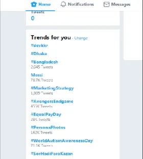
Trends in Twitter- Twitter itself has a facility to show what sort of trends are right now drifting around the world. The algorithm used by twitter, by default they are tailored for

Figure 3.1.1: Trend list of Twitter on April 3, 2019

(19)

9

the user, based on the user’s following list, his/her hobbies or interests, and the user’s location. This algorithm identifies topics that are popular right now, rather than topics that have been popular for a while.

It helps the user to discover the latest trendy topic which is being discussed on Twitter.

Trends usually vary by a big margin during a significant event or program. Such as- It is pretty obvious that during the Olympic or Football world cup, the trendiest topic on the discussion platform will be on those events.

Hashtags- A word or phrase started with this sign ‘#’ is usually denoted as hashtags. They usually deliver the gist of the main interest of the tweet that has been tweeted. For example- #RealVSBarca, #ElClassico, #World_climate_day. These hashtags must be a single set of strings. There are no whitespaces between two different words. They can be separated by using underscore’_’, but whitespaces break the tag.

The trends have been a good indicator of the situation of the current global events and incidents lately. The impact of the trends has been enormously observed for the last couple of years. Some recent political, socio-economical events have been on the trend list and mostly all of them came up with their own trendy hashtag. For instance- the movement against the sexual assault against women in the workplace had come to light with a hashtag called “#metoo” and an enormous number of women have shared their horrific experiences with this hashtag including some well-known popular women around the globe. We are also aware of another international issue that is Britain exiting the European Union and it's been called “Brexit”. This hashtag has also caught attention for the last couple of years.

These events implicate the wide impact of trends and hashtags these days.

3.2 Research Subject and Instrumentation

In this section, we will describe the terms and the theories that are necessary for our research.

Time Series: In an event of a regular occurrence of data in some different intervals of time, a correlation is established between time and the statistical modeling. And “the systematic

(20)

10

approach by which one goes about answering the mathematical and statistical questions posed by these time correlations is commonly referred to as time series analysis”[9].

In simpler words, “Time series is a sequence of observations recorded at regular time intervals” [7].

A time series can be different intervals of time such as hourly, daily or even monthly. In some cases of short-term analyzing, it can also be minute or second-wise. For example, to analyze the stock market price, every minute of data is recorded.

Time series modeling is very efficient to identify and locate existing patterns in repetitive data and predict the future occurrence of those data by using them. One of the most exquisite features of time series modeling is that it’s very much budget-conscious than the other analytical solutions but it will provide strong insights.

Typically, time series analysis follows two primary goals or aims. Those are-

▪ Pointing out the pattern of a series of observations.

▪ Giving prediction of the future occurrence using the observations, which is commonly called forecasting.

There are five types of traditional time series models most commonly used in epidemic time series forecasting [5]and those are-

1.

Autoregressive (AR), 2. Moving Average (MA),

3. Autoregressive Moving Average (ARMA),

4. Autoregressive Integrated Moving Average (ARIMA)

5. Seasonal Autoregressive Integrated Moving Average (SARIMA)

(21)

11

ARIMA Model: To get acquainted with the basic concept and implementation of the ARIMA model, we need to illuminate another term which is “Stationarity”. In a time series dataset, the data are a function of time. With time, data can be seasonal or trendy. This means in a time series model, there can be data recur over a regular period of time which is called seasonality or there can be data which are called trends, in other words upward or downward movements in the dataset. Fixing these issues and making data independent from the function of time is called making data stationary.

For a non-stationary time series, it has to be transformed into a stationary initially.

“ARIMA model usually fits the non-stationary time series based on the ARMA model, with a differencing process that effectively transforms the non-stationary data into a stationary one”[5].

An important point to observe here is that ARIMA works better when the data is stationary.

That means when there is no seasonality or trend. Also, ARIMA requires a parameter series that can be calculated based on the dataset. Those are some constraints of ARIMA.

RNN LSTM: The Neural Network is the compound of a massive number of interconnected processing elements or neurons that work combinedly to solve any given tasks. A neural network learns from experiences and mistakes, just as a human being.

In a neural network, there are three basic layers.

1. Input Layer 2. Neurons 3. Output Layer

A traditional neural network has a shortcoming of understanding events with the help of previous events. The RNN fixes that issue. It runs loops within the network allowing them to persist[18].

(22)

12

RNN is called Recurrent Neural Network because it performs identical operations for each output of information whereas the output of the present input depends on the computation of the previous one. After generating the output, it is derived and sent into the recurrent network

RNN can use their internal state or memory to learn from the previous states. In RNN, all

the inputs are connected with each other. This is what happens inside of a recurrent neural network. Here, the Xt is the input and A is the activation layers that generate ht or the output. Initially, the layer takes X(0) from the sequence of the input and generate the output h(0). They are the inputs of the next step together and it goes on. This is how the network functions and finally generates the output.

Unfortunately, there is a shortcoming in RNN. That is called Long-term dependencies.

Which states that RNN is unable to learn to connect the information between two long gaps of the neurons or memories. That is why LSTM is introduced.

“Long Short Term Memory network or “LSTM” – is a special kind of RNN, capable of learning long-term dependencies. LSTMs are explicitly designed to avoid the long-term dependency problem”[18].

In our model, we used the Long-Short Term Memory method also known as LSTM of Recurrent Neural Network. There is a definite reason for that. It’s been already mentioned above that ARIMA requires a series of parameters to function. On the contrary, LSTM does not require such kind of parameters. It’s also required that the dataset for ARIMA to

Figure 3.2.1: Workflow of an RNN model[18]

(23)

13

apply need to be stationary. This means it needs to deprived of trend and seasonality which is not required for our dataset.

Besides that, ARIMA is popular for time series analysis whereas LSTM is not quite explored enough in this sector comparatively. That makes it a good area for researching and one of the reasons for picking LSTM over ARIMA.

To create a suitable environment to conduct our research, the requirements are needed to mention initially. So below is a list of the tools and languages that we used throughout our research-

▪ Programming Language: Python

▪ Python Libraries: Pandas, Numpy, Scipy, matplotlib, sklearn

▪ Environment: Tensorflow 2.0

▪ Streamer: Tweepy

3.3 Data Collection Procedure

In any research, dataset plays a key role. We could not use any sort of existing dataset as our research is based on real-time streamed tweets and hashtags. So with twitter’s API, we streamed tweets and saved them in a CSV file. Later, we isolated the specific hashtag that we are going to train our model on and saved its counts in an SQLite database. To proceed further, we need to explain the nature of our dataset because there are some explicit distinctive features between a regular dataset and a time-series dataset.

3.3.1 Time Series Dataset Nature

To work with time series data, we need to understand the behavior and characteristics of a time series dataset. It is already established from our discussion and definitions above that to be in a time series dataset, a data must occur in a regular interval of time, thus making it time series data.

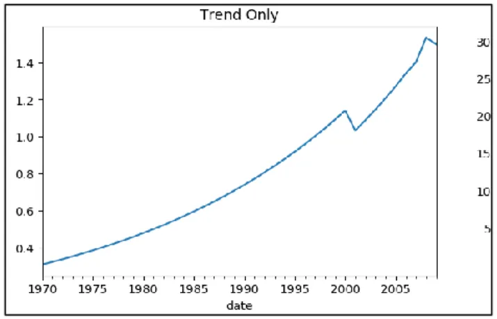
“A time series data can be split into four basic components, those are- Base Level, Trend, Seasonality, and Error”[7]. A trend is identified when an increment or decrement is

(24)

14

observed within the slope of the time series. Seasonality is identified when a pattern is repeated between regular intervals on account of seasonal factors such as- during Christmas, the sale of the Christmas trees hits a hike.

In a time series dataset, only one or even both type of attributes can be present. It depends on the dataset. Below, the types are presented in different graphs for different sorts of datasets-

Figure 3.3.1.1 is a dataset of guinea ice, where the trend is identified only. Here the production seems to upward with the time, which means a trend has been observed.

Whenever there is an upward or downward movement is observed in a time series dataset, it can be determined that a trend is present there.

Figure 3.3.1.1: A dataset where only trend is present[11]

Figure 3.3.1.2: A dataset where only seasonality is present[12]

(25)

15

Figure 3.3.1.2 is a dataset of some areas of sunny spots such as beaches. As we can observe, the summer season is the key attribute here. Hence, during the summer, the population of those areas is incrementing, and afterward, it decreases. Which means it follows the seasonality.

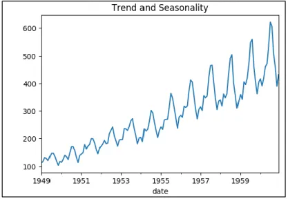
Figure 3.3.1.3 is a dataset of the air passengers of an airline. As we can see, both attributes, trend as well as seasonality, are observed here.

Figure 3.3.1.3: A dataset where trend and seasonality both are present[13]

(26)

16

The dataset we used, belongs to the latter category. In our dataset, both trend and seasonality are present. Initially, we opened a developer account on twitter to obtain authentication keys from twitter to stream tweets. The next step after acquiring the credentials was to start importing tweets and saving it in a CSV file for further analysis.

We used “Tweepy”, a python library to access the twitter’s API. It provides multiple facilities as follows- importing tweets from the accounts we follow, importing tweets from our own accounts and etc. We isolated those tweets with hashtags from those which don’t have any hashtags, then saved the account name, the tweet and the hashtag in the CSV file.

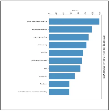
Further, we counted the frequency of each hashtag and later plotted them in a bar chart for visualization of the counts. For instance- following is the hashtag count from Twitter on April 3rd,2019-

On that particular month, the biggest grossing movie of the history “Avengers: Endgame”

was released. So, it is no surprise that it was in the first position of the most trendy hashtag on twitter. In the figure above we showed only the first 10 hashtags with the most appearance. This was just a test run to check if our streaming was working accordingly.

Figure 3.3.1.4: Hashtag count on April 3, 2019

(27)

17

Our aim was to determine the frequency shifting of the trends for a specific community.

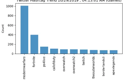
We chose the gaming genre for our research. On October 25^th of 2019, one of the most popular gaming franchises of all time, Call of Duty, was set to release its latest installment, Call of Duty: Modern Warfare(2019). This was a golden opportunity for us to conduct our research as this game is part of one of the highest-grossing game series of all time. The following is the streamed hashtag count of some game name tags on 29^th October. 2019-

To study the pattern of the trend, we needed to observe its ups and downs throughout a long period. So we started our streaming from Twitter from October 4^th and concluded on October 28^th. That’s because, to train our model, we can’t feed a chunk of data with only the highest count of the trend. We needed to make it learn to determine the pattern that lies in the trend. So we tried to capture the uprising of the trend so that our model can forecast just precisely as it could. In the total period of twenty-four days of streaming, we streamed by 8 sessions with three hours of interval. Each session continued for approximately 15 minutes. The tweets were restored in a CSV file at the beginning with the text of the whole tweet, the username of the tweet and all the corresponding hashtag with that particular

Figure 3.3.1.5.: Hashtag count of game names on October 29^th, 2019

(28)

18

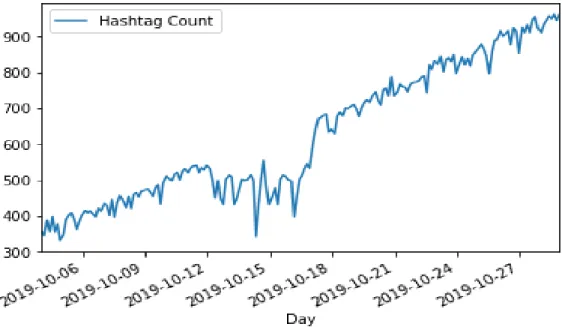
tweet. Following is the graphical representation of the count of our trend hashtag

“modernwarfare” for 24 days-

In the figure above, the hashtag count of ‘modernwarfare has been taken from October 4^th to October 28^th.

Figure 3.3.1.6: Graphical representation of the hashtag count modernwarfare for 24 days

(29)

19

3.4 Statistical Analysis

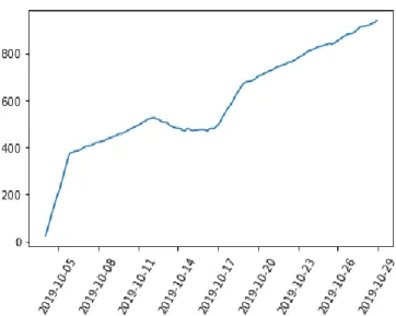
We can also visualize the characteristic of our dataset from some more reliable and popular methods. Below is the box plotted visualization of our dataset, where both trend and seasonality have been shown together-

In figure counted, a small setback can be observed in the hashtag counts dataset. That can be caused by many reasons. “Noisy data can be caused by hardware failures,

programming errors and gibberish input from speech. Spelling errors, industry abbreviations as well as slang can also impede machine reading” [20].

In case of the presence of noisy data, data smoothing is required for the model to perform up to the mark. “Data smoothing is a statistical technique that involves removing outliers from a data set in order to make a pattern more visible” [19]. Smoothing the dataset can pave the way to a content forecasting learning model.

So, we tried to smooth our dataset as well and we used two library functions for that for a better outcome. Primarily we imported the ifilter function from scipy library and obtained the following output-

Figure 3.4.1: Box plot representation of the dataset

(30)

20

But this is a bit sporadic in the middle. So, for a better outcome, we further imported savgol_filter. It generated the outcome below-

With this outcome, now we can proceed to build a smooth model for better forecasting of the test data.

Notwithstanding, one crucial issue should be aforementioned here. That is, however,

“data smoothing can overemphasize certain data and ignore other data.”[19].

Figure 3.4.2: Smoothened data using ifilter

Figure 3.4.3: Smoothened data using savgol_filter

(31)

21

3.5 Implementation Requirements

After importing our dataset with pandas library, the very first thing we needed to do was to index the data. This means, in the dataset, there are two columns. One is for the DateTime and the other one is the count of the tweet for that particular time. Hence, we needed to index the DateTime column and convert its format to DateTime from string.

Thereafter, we divided the into training and testing list with the train test split function.

There were in total of 192 rows of data in our dataset. That means 192 reading of the hashtag count occurring through regular intervals of time for 24 days. In our training section, we added 176 rows and in our test section, we added the rest 16. Now, one important issue is mentionable here that is, when we applied the fit function at the end of our model, we didn’t apply it to the test data. That’s because we want to attempt to predict these 16 rows or 2 days of data, using only the training data we had so that we will be able to compare our generated 2 days to our actual true historical values from the test set.

3.5.1 Data Normalization: Min- Max Scaler

The next thing we needed to perform was to normalize the data. “Normalization squeezes the data between 0 and 1, these smaller values could flow easily through our neural network without giving any weird predictions”.[14]

There are many formulas and techniques for data normalization. One of the most popular is Min- Max scaler. It follows-

𝑋_𝑛 = 𝑋 − 𝑋_𝑚𝑖𝑛

𝑋_𝑚𝑎𝑥− 𝑋_𝑚𝑖𝑛 ( 1 )

This scaler transforms all the data into the range of 0 to 1.

(32)

22

3.5.2 Batch Function

The basic aim of training the dataset with batches is to enhance the speed of learning. If the data is processed as a whole, it can slow down the process. Hence, the dataset is passed through the neural network as batches which are just a small subset of the entire training dataset.

The purpose of splitting the Dataset into batches is typically to speed up the learning.

Instead of processing the entire set of training examples, it processes only a batch, which is just a small subset of the entire training set, at a time. There are various techniques about how to formulate such batches and process them to get the final trained model.

The batch function that we built for our model had training data, batch size and time steps for each batch as input and later it returned a tuple of y time series results as the output.

3.5.3 RNN LSTM Model with TensorFlow

The RNN LSTM model that we built for our research is solely compounded with three basic fragments. Initially, there are the constants of the model. Following, the loss function and optimizer. Subsequently, session initializer to process the batch functions that we discussed above.

3.5.4 The Constants of the LSTM Model

As we have mentioned above, we used the LSTM method of Recurrent Neural Network (RNN). To build the model, we needed to define some constants initially. The value and the descriptions for those constants are given below-

(33)

23

The number of inputs here is just one, the time series. Then the number of steps in each batch is 16. Afterward, we defined the number of neurons per layer to 200. This is not a fixed value, it depends on the outcome of the model. For our case, we obtained a satisfactory result by setting it to 200 after multiple iterations. Next, our output. In this case, there is only one output, the prediction. Thus, it is set to 1. The learning rate is set to 0.001. Following that, iterations for training are 6000 which indicates how many training steps will go through. Finally, the batch size, that indicates how many batches will go through the model in every iteration. We set it to 1.

3.5.5 Loss Function & Optimizer

The loss function is the process for the machine to learn. In an LSTM model, a loss function is a method to evaluate how much specifically the algorithm is modeling the given dataset.

If the loss function produces a higher number, then it indicates that the predicted value is too much deviating from the actual values. The optimizer function helps the loss function to reduce the errors in the outcome.

“Loss functions can be classified into two major categories depending upon the type of learning task we are dealing with — Regression losses and Classification losses”[21]. Our dataset belongs to the latter category, that is Regression. Regression deals with the data that

Name of the Constant Value of the Constant

Inputs 1

Time Steps 16

Neurons per layer 200

Outputs 1

Learning Rate 0.001

Iterations for training 6000

Batch Size 1

Table 3.5.4.1: Constants of LSTM model

(34)

24

are continuous such as- given previous week’s record, predicting the stock market points for the next day.

In our model, we used mean square error loss function and Adam optimizer. Mean square error also known as MSE is “measured as the average of the squared difference between predictions and actual observations”[21]. Following, “Adam is an optimization algorithm that can be used instead of the classical stochastic gradient descent procedure to update network weights iterative based on training data”[22].

(35)

25

CHAPTER 4

Experimental Results & Discussion 4.1 Experimental Results

As we have mentioned above, we will not be fitting our test data to the fit function because we don’t want to let the model know about the future. So, to predict two days of data i.e 16 rows, we will feed in a seed training_instance of the last 2 days of the training_set of data to predict 2 days into the future. Then we will be able to compare our generated 2 days to our actual true historical values from the test set.

After generating the count, we ran an inverse scaler to re-transform the data into its original shape. Then we put that result into a generated column on the dataset.

Afterward, we plotted the two-column, the actual count and our predicted count in a graph to visualize the difference-

Figure 4.1.1: Actual hashtag count vs predicted hashtag count

(36)

26

4.2 Descriptive Analysis

In a time series analysis, there are a few obsolete ways to measure accuracy. But it is better to measure the errors in the series with respect to the actual values. Our test dataset contained 16 rows of data or 2 days of data. We smoothened our training dataset, leaving the test dataset unharmed and unchanged as we want to compare our prediction with the actual raw data.

There are multiple methods to measure error. One of them has been already applied and described under the loss function and optimizer section. In this part, we used another popular method to measure the error that is Absolute Forecast Error. The formula of the error is following-

MAE =

∑(𝑎𝑏𝑠( 𝑎 – 𝑝))

𝑙𝑒𝑛(𝑎)

( 2 )

Here, MAE stands for Mean Absolute Error. A is the actual value, P is the predicted value.

The abs function is obtaining the absolute value of the difference between them. Then we find their mean by summing consequently and dividing them by the total number of the actual values that are present. The table representation is given below-

(37)

27

Entry Absolute Forecast Error

Actual Value

Predicted Value

0 66.309998 854 920.309998

1 0.190308 925 924.809692

2 18.227173 911 929.227173

3 0.576294 933 933.576294

4 26.856262 911 937.856262

5 2.930969 945 942.069031

6 8.785461 955 946.214539

7 27.286926 923 950.286926

8 43.281128 911 954.281128

9 24.195251 934 958.195251

10 17.028809 945 962.028809

11 8.780579 957 965.780579

12 20.450745 949 969.450745

13 12.009644 961 973.009644

14 31.395874 945 976.395874

15 19.590942 960 979.590942

From the table above, we obtained that our mean absolute error = 20.4935

4.3 Summary

It is hard to say if the model is accurate or the error rate is sufficiently less as there is no benchmark for the forecasting error or accuracy for time series models. Our dataset was collected within a short period and they changed drastically as well because of their context and importance. That is why our research has its flaws to work on and to improve.

However, for now, this is the best result we could generate with our limited equipment and time.

Table 4.2.1: Absolute forecast error of the model

(38)

28

CHAPTER 5

Summary, Conclusion, Recommendation and Implication for Future Research

5.1 Summary of the Study

Trends are at present one of the crucial indicators of modern society. It is the indicator of changing issues, the inflow of the discussion topics. In multiple aspects of our life, we have converged our lifestyles with trends. From fashion to food, business to sports, technology to entertainment, we like to keep ourselves updated with the concurrent world. This nature of ours has played a vital role to find the impact of our research. As we have mentioned earlier that our research is dedicated to analyzing trends for a specific community, we are going to discuss the impact of trends in certain sectors.

5.1.1 Trends in Business

Perhaps one of the crucial role that our research can play on is the business sector. The industry is fast-paced, changing its tactics every day. Because of technological advancement, it has become more competitive and complicated. The data of the consumers are playing a decisive role as this era has shown an enhancement in big data analysis. The pattern in consumer behaviors is pivotal. A product’s price can fluctuate upon the decisions of the consumers. So it is extremely crucial to monitor the trends and finding a pathway to establish a correlation between the products and the customers by using the trends.

In recent days, a fantastic approach to marketing has caught our eye that is directly relevant to our research. Marketing is one of the main feature of any business to shoutout one’s products to the corresponding consumers. Recently, we are all aware of the price hike in onion’s market. It has been criticized, discussed all over the country. For quite some time, it has remained one of the major trendy issues of the country. We have observed that some business company has taken this chance and done marketing stunt using this trend. The advertising they posted on their facebook page was following-

(39)

29

The noticeable fact here is that the company has used the concept of “people love to follow trends” and they used it for the marketing of a completely different product that is motorbikes. Judging the number of likes, comments as well as sharing, this ad engaged more people than the other usual ads of the page.

Another marketing policy that we observed was by one of the most popular online shopping portals of our country, Daraz. It follows-

Figure 5.1.1.1: Advertise of evaly posted on the facebook page[17]

Figure 5.1.1.2: Advertise of daraz posted on the facebook page[16]

(40)

30

At the beginning of October, a worldwide acclaimed movie “Joker” was released. It was one of the most hyped movies of this year. So, people started to follow this trend typically.

Daraz took that chance and did a marketing boost by connecting themselves with that trend.

These are just small fragments of how the following of the trends can play an extremely crucial role in business policy.

5.1.2 Trends in Technology

Technology has been one of the fastest-growing sectors of the 21^st century. Every single day it is continuing to amaze us. It is futile to discuss the necessity of following the trends in this field as this particular genre itself is one of the trendsetters of the world, From cellphones to android os, nano-tech, biotechnology, technology never ceases to astonish us with its new inventions. Those who do not keep themselves updated with the trends and latest technologies these days are considered to be backdated. Hence, trend analysis for the tech freaks can be proven quite crucial. Being members of a global village, the people of the world are now more connected with each than they ever were. The trends that we follow from here, can easily be tracked from a remote corner of the world by the blessings of technology.

5.2 Conclusion

The purpose of any research is the practice of analytical mind, improving and acquiring a sound knowledge on field, discovering a new approach to a problem. Ours was not any different. Trends have been a common and burning issue in our country for the last couple of years. People tend to follow and discuss trendy topics in social media so often. This behavioral pattern caught our eye and with our newly gained knowledge of machine learning, we tried to analyze and explore this seemingly interesting field. To conclude, trend analysis can play a key role in multiple daily life sectors as well as research fields.

Our research was dedicated to analyze the pattern of the trends for a particular community.

This study of trends can assist those communities to keep track of their favorite hashtags on Twitter.

(41)

31

5.3 Recommendations

Trend analysis can not only have impacts on pragmatic fields, it can also lead to new research sectors. Because it fundamentally depends on the behavior of people, how they respond to a growing topic. This study can lead to behavioral analysis, sentimental analysis, the relevance of an issue and so on. In this era of machine learning with big data analysis, these research fields can be a major key to establish a more advanced relationship between machine and human.

5.4 Implications for Further Study

For further study, we have decided to conduct our research on facebook in the future as it is the most popular social media in the entire world. But there can be multiple issues that can arise such as text summarization, topic classification, text scrapping. There are multiple research fields only dedicated to these studies. Our aim will be studying those fields and establish a sound correlation between those fields and our findings from this research.

(42)

32

Appendix

Following is the figure of the SQLite database entries of the counts of the hashtags at the beginning of the month October when the count of #modernwarfare was comparatively low-

Following is the figure of the SQLite database entries of the counts of the hashtags at the ending of the month October when the count of #modernwarfare was comparatively high-

Figure A1: Counts of hashtags in SQLite on the beginning of the month October

Figure A2: Counts of hashtags in SQLite on the ending of the month October

(43)

33

References

[1] “Tweeting Made Easier,” Twitter. [Online]. Available:

https://blog.twitter.com/official/en_us/topics/product/2017/tweetingmadeeasier.html. [Accessed: 14-Oct- 2019].

[2]"Global social media ranking 2019 | Statistic", Statista, 2019. [Online]. Available:

https://www.statista.com/statistics/272014/global-social-networks-ranked-by-number-of-users/. [Accessed:

02- Apr- 2019].

[3] "How Much Time Do We Spend On Social Media? [Infographic]", Mediakix | Influencer Marketing Agency, 2019. [Online]. Available: http://mediakix.com/2016/12/how-much-time-is-spent-on-social-media- lifetime/#gs.3ku4a0. [Accessed: 02- Apr- 2019].

[4] "TREND | meaning in the Cambridge English Dictionary", Dictionary.cambridge.org, 2019. [Online].

Available: https://dictionary.cambridge.org/dictionary/english/trend. [Accessed: 02- Apr- 2019].

[5] S. Chatterjee, “ARIMA/SARIMA vs LSTM with Ensemble learning Insights for Time Series Data,” Medium, 13-May-2019. [Online]. Available: https://towardsdatascience.com/arima-sarima-vs-lstm- with-ensemble-learning-insights-for-time-series-data-509a5d87f20a. [Accessed: 14-Oct-2019].

[6] “Time Series for Dummies – The 3 Step Process,” KDnuggets. [Online]. Available:

https://www.kdnuggets.com/2018/03/time-series-dummies-3-step-process.html. [Accessed: 14-Oct-2019].

[7] “Time Series Analysis in Python - A Comprehensive Guide with Examples – ML,” Machine Learning Plus, 14-Feb-2019. [Online]. Available: https://www.machinelearningplus.com/time-series/time-series- analysis-python/. [Accessed: 14-Oct-2019].

[8] E. Lisowski, “The best Forecast Techniques or how to Predict from Time Series Data,” Medium, 23-May- 2019. [Online]. Available: https://towardsdatascience.com/the-best-forecast-techniques-or-how-to-predict- from-time-series-data-967221811981. [Accessed: 14-Oct-2019].

[9] R. H. Shumway and D. S. Stoffer, Time series analysis and its applications: with R examples, 4th ed.

New York: Springer, 2017.

[10] “Time Series and Forecasting Formula,” Time Series and Forecasting Formula.

[Online].Available:https://origin2.cdn.componentsource.com/sites/default/files/resources/dundas/538216/D ocumentation/Forecasting.html. [Accessed: 15-Oct-2019]

[11] The world's leading software development platform · GitHub. [Online]. Available:

https://raw.githubusercontent.com/selva86/datasets/master/guinearice.csv. [Accessed: 17-Oct-2019].

https://raw.githubusercontent.com/selva86/datasets/master/sunspotarea.csv. [Accessed: 17-Oct-2019].

https://raw.githubusercontent.com/selva86/datasets/master/AirPassengers.csv. [Accessed: 17-Oct-2019].

[14] S. Panchal, “Normalization of Crazy Data - Python,” Medium, 16-Oct-2018. [Online].

Available:https://medium.com/@equipintelligence/normalization-of-crazy-data-python-4fa6611e7b46.

[Accessed: 17-Oct-2019].

[15] "Video game industry", En.wikipedia.org, 2019. [Online]. Available:

https://en.wikipedia.org/wiki/Video_game_industry. [Accessed: 29- Oct- 2019].

[16] "Daraz Online Shopping", Facebook.com, 2019. [Online]. Available:

https://www.facebook.com/DarazBangladesh/photos/a.1706977462860779/2969417259950120/?type=3&t heater. [Accessed: 30- Oct- 2019].

[17] "evaly.com.bd", Facebook.com, 2019. [Online]. Available:

https://www.facebook.com/evaly.com.bd/photos/a.1885516608177724/2592095130853198/?type=3&theat er. [Accessed: 30- Oct- 2019].

(44)

34

[18] "Understanding LSTM Networks -- colah's blog", Colah.github.io, 2019. [Online]. Available:

https://colah.github.io/posts/2015-08-Understanding-LSTMs/. [Accessed: 01- Nov- 2019].

[19] "Data Smoothing Definition & Example | InvestingAnswers", Investinganswers.com, 2019. [Online].

Available: https://investinganswers.com/dictionary/d/data-smoothing. [Accessed: 02- Nov- 2019].

[20] "What is noisy data? - Definition from WhatIs.com", SearchBusinessAnalytics, 2019. [Online].

Available: https://searchbusinessanalytics.techtarget.com/definition/noisy-data. [Accessed: 02- Nov- 2019].

[21] R. Parmar, "Common Loss functions in machine learning", Medium, 2018. [Online]. Available:

https://towardsdatascience.com/common-loss-functions-in-machine-learning-46af0ffc4d23. [Accessed: 03- Nov- 2019].

[22] J. Brownlee, "Gentle Introduction to the Adam Optimization Algorithm for Deep Learning", Machine Learning Mastery, 2017. [Online]. Available: https://machinelearningmastery.com/adam-optimization- algorithm-for-deep-learning/. [Accessed: 03- Nov- 2019].

[23] A. Kaplan and M. Haenlein, "Users of the world, unite! The challenges and opportunities of Social Media", Business Horizons, vol. 53, no. 1, pp. 59-68, 2010. Available: 10.1016/j.bushor.2009.09.003.

[24] P. Liu, Mining Social Media: A Brief Introduction. INFORMS TutORials in Operations Research, 2014.

[25] S. Hendrickson, J. Kolb, B. Lehman and J. Montague, "twitterdev/Gnip-Trend-Detection", GitHub, 2019. [Online]. Available: https://github.com/twitterdev/Gnip-Trend- Detection/blob/master/paper/trends.pdf. [Accessed: 28- Nov- 2019].

[26] Cvijikj, Irena Pletikosa, and Florian Michahelles. "Monitoring trends on facebook." 2011 IEEE Ninth International Conference on Dependable, Autonomic and Secure Computing, IEEE. pp. 895-902, Dec 2011.

[27] Bhulai S, Kampstra P, Kooiman L, Koole G, Deurloo M, Kok B. “Trend visualization on Twitter: what’s hot and what’s not?” Data analytics. 2012. pp.43-8, 2012.

[28] Mathioudakis, M., & Koudas, N. (2010, June). “Twittermonitor: trend detection over the twitter stream.”

2010 ACM SIGMOD International Conference on Management of data, ACM.. pp. 1155-1158, 2010.

[29] Jeon, Seungwoo, Bonghee Hong, Juhyeong Kim, and Hyun-jik Lee. "Stock Price Prediction based on Stock Big Data and Pattern Graph Analysis." IoTBD, pp. 223-231. 2016.

[30] Pavlyshenko, Bohdan M. "Machine-learning models for sales time series forecasting." Data 4, no. 1, pp 15, 2019.

[31] Mudinas A, Zhang D, Levene M. “Market trend prediction using sentiment analysis: lessons learned and paths forward.” arXiv preprint arXiv:1903. 05440. Mar 2019.

(45)

35