The Comparison of Classical and Bayesian Bivariate Binary Logistic Regression Prediction for Unbalanced Response (Case Study: Customers of Antivirus Software 'X' Company)

(1)

THE COMPARISON OF CLASSICAL AND BAYESIAN

BIVARIATE BINARY LOGISTIC REGRESSION

PREDICTION FOR UNBALANCED RESPONSE

(

CASE STUDY: CUSTOMERS OF ANTIVIRUS SOFTWARE 'X' COMPANY

)

Muktar Redy Susila, Heri Kuswanto, Kartika Fithriasari

Faculty of Mathematics and Natural Science, Insitut Teknologi Sepuluh Nopember

1D/14A Sukolilo, Surabaya 60111, Indonesia

muktarredys@gmail.com (Muktar Redy Susila)

Abstract

The purpose of this study was to compare the performance of classical bivariate binary

logistic regression and Bayesian bivariate binary logistic regression. The sizes of sample used

in research were small and large sample. The size of the small sample was 200 and the large

sample was 10000 samples. Parameter estimation method that often used in logistic

regression modeling is maximum likelihood which is called the classical approach. However,

using a maximum likelihood parameter estimation has several weaknesses. When the number

of sample is small and the dependent variable is unbalanced, bias parameters are frequently

obtained. Nevertheless, when the sample size is too large, it has propensity to reject H

0

. As

the solution, the use of Bayesian approach to overcome the small sample size problem and

unbalanced dependent variable is suggested. The case study carried out in this research was

customer loyalty of 'X' Company. This study used two dependent variables, i.e. Customer

Defections and Contract Answer. Initial information on the number of consumers who

defected and not defected was unbalanced, likewise for the Contract Answers. Based on the

comparison of classical and Bayesian bivariate binary logistic regression prediction, Bayesian

method was evidenced to yield better performance compared to classical method.

Keywords: binary logistic regression, Bayesian, classical, unbalanced, bivariate.

Presenting Author’s biography

(2)

1.

Introduction

Customer loyalty is an indicator of the performance of a given company. The factors related to the product can affect customer loyalty. Analysis and detection of customer loyalty is required to maintain the performance of a company. Detection of customer loyalty can be done by predicting customer loyalty based on the factors that influence it. The 'X' Company is an organization that provides antivirus products and operates by using internet connection system. The 'X' Company is currently working with contract system and completing customer loyalty issues. It is working with contract system and having customer loyalty issues. To obtain an overview of the company criteria on loyal customer, it is not possible to approach the customers directly. With this constraint, the company can use the available information. Based on available information, the criteria and prediction on customers’ loyalty can be figured out.

Previous studies preoccupied on customer loyalty in the 'X' Company have been carried out by Kanamori, Martono, Ohwada, and Okada [1], Martono and Ohwada [2], and Martono [3]. The methods used in those studies were based on Machine Learning. Machine Learning method, however, failed to statistically interpret the relationships between the predictor variable and response variable. In addition, Asfihani [4] carried out a research by using binary logistic regression and Lorens method. The data used in the study was unbalanced dependent variable and the result obtained bias parameter. While Lorens method could not be interpreted statistically.

Generally, the weakness of previous studies was on the indicator of customer loyalty which was Customer Defection. Five independent variables (predictors) were used in previous studies, i.e. Contract Answer, Accumulation of Renewal, Price of Product, Type of Costumer, and Status of Email Delivery. Ideally, to answer customer loyalty problems, Contract Answer should be used as a dependent variable (response). There is one-year relationship contract between the company and the customer. Regularly, the company sends notification of the auto-renewal update for each customer by e-mail in the period between fifty to zero days of product expiration. By receiving the e-mail notification, the options for the customer is to “opt-in” or “opt-out”. In the case the customer chooses to opt-in, it indicates positively that they would like to be contacted with a particular form, in this case with a renewal form. On the contrary, the preference of opt-out indicates that they would prefer not to be in, or in other words, it is a form of defection and customer can move to other products of the company. Thus, this study used two dependent variables, namely Customer Defections and Contract Answer.

To improve the performance of the 'X' Company, information on the factors that affect customer loyalty is required. The relationship between Customer Defections and Contract Answer are interrelated. Initial information about the number of consumers who defected and not defected is unbalanced, likewise for the Contract Answers. Contract Answers variable is rare events in which the answer to continue the contract is considered to be very rare.

Logistic regression is one of the models used for prediction or classification. This model can indicate factors that significantly influence the dependent variable. Binary logistic regression modeling is generally performed on the data with one dependent variable. According to McCullagh and Nelder [6] binary logistic regression model which has two interrelated dependent variables can be modeled into a model called bivariate binary logistic regression. The binary regression model is used to explain the probability of a binary response variable as a function of some covariates. According to Ali, Darda, Holmuist [7] bivariate logistic regression is a useful procedure with advantages that include individual modeling of the marginal probability distribution of the bivariate binary responses, and modeling the odds ratio describing the pairwise association between the two binary responses in relation to several covariates.

Parameter estimation method often used in logistic regression modeling is maximum likelihood. This model is called the classical approach. However, using a maximum likelihood parameter estimation has some weaknesses. When the number of sample is small and the dependent variable is unbalanced, bias parameters are often obtained [8]. According to Schaefer [9] the small sample size is under 200

(3)

tends to identify P-value as close to 0. Classical approach is frequently ineffective when the sample size is too large due to its ambiguous result. Dumouchel [11] suggests the use of Bayesian approach to overcome the small sample size problem and unbalanced dependent variable.

Basically, the purpose of this research was to compare classical and Bayesian bivariate binary logistic regression prediction. This research involved small and large sample size. The sample size for the small sample was 200 samples and the large sample was 10000 samples.

2.

Methods

2.1 Bivariate binary logistic regression model

Bivariate binary logistic regression is a development of binary logistic regression. In the beginning, binary logistic regression modeling has only one dependent variable. Along the development of a binary logistic regression, the modeling could be done for more than one dependent variable. For two dependent variables, it was called bivariate. So, the binary logistic regression which has two interrelated dependent variables is called bivariate binary logistic regression [12]. Let define two

binary dependent variables

(

Y₁

,

Y₂

)

, which the variables Y₁ and Y₂ expressed an event 'success' or

'failure', then the event can be modeled by bivariate binary logistic regression.

Tab. 1 The probability for bivariate observation

1

Y

2 Y

0 1 Total

0

00

p p₀₁ 1-p₁

1

10

p p₁₁ p₁

Total

1-2

p p₂ 1

In Table 1, prs= P(Y1=r Y, 2=s), r, s = 0, 1 are the joint probabilities and pj =P(Yj =1), j =1, 2 is

the marginal probabilities for each response variables. It is assumed that the observations within pairs

are correlated but observations from different pairs are independent. When there are m independent

variables x x1, 2,...,xm then the value p p1, 2,...,pm are:

01 11 1 1

1

01 11 1 1

exp( ... )

( )

1 exp( ... )

m m

x x

p x

x x

β β β

+ + +

=

+ + + +

(1)

02 12 1 2

2

02 12 1 2

exp( ... )

( )

1 exp( ... )

m m

x x

p x

x x

β β β

+ + +

=

+ + + +

(2)

Bivariate binary logistic regression models can be expressed from logit p x₁( )and logit p x₂( ) which

is a linear function of

β

₁TX and

β

₂TX

, with

[

]

1 01, 11, 21,..., m1

β = β β β β

(3)

[

]

2 02, 12, 22,..., m2

β = β β β β

(4)

[

0, ,1 2,...,

]

T m

X = x x x x

(5)

ψ

is an odds ratio that shows the relationship between the variables Y₁ and Y₂,

11 00

10 01

, 0

π π

ψ ψ

π π

(4)

where Y₁ and Y₂ are independent ψ =1. The value of log

is

ψ

=

�, with θ γ= TX

,

where

γ

is a bound

parameter vector. The joint probabilities p₁₁ according to Dale [13] and Palmgren [14] can be

obtained in terms of p1, p2, and ψ as

(

)

1

{

2

}

1 2

1

1 , 1

2

, 1

a a b

ψ ψ ψ π π ψ −  ₋ ₋ ₊ _≠  =   ₌ 

(7)

The other three joint probabilities can be recovered easily from the marginalp₁₀ = p₁−p₁₁,

01 2 11

p = p − p , and p00= −1 p10−p01−p11.

2.2 Parameter estimation using maximum likelihood method (classical bivariate binary logistic regression)

Maximum likelihood method requires that parameters appraising must know the distribution of the

model. The maximum likelihood method works by maximizing the likelihood function. If n random

sample of observations are scaled on bivariate binary data, then the bivariate random variables(Y₁i,

2i)

Y i = 1, 2, 3,…,n will be identical with (Y₁₁_i,Y₁₀_i,Y₀₁_i,Y₀₀_i). They have multinomial distribution

with probabilityp11i, p10i, p01i, p00i. So, the likelihood of a bivariate random variable is as follows:

1

11 11 10 10 01 01 00 00 0

( ) P( _i _i, _i _i, _i _i, _i _i)

i

L Y y Y y Y y Y y

=

∏

= = = =

β

11 10 01 00

11 10 01 00 1

i i i i

n

y y y y

i i i i

i

p p p p

=

∏

(8)

The parameterβ=(β , β ,θ  1 2 )is obtained by maximizing the equation (8) by derive it to its parameters.

11 10 01 00

11 10 01 00 1

ln ( ) ln i i i i

n

y y y y

i i i i

i

L p p p p

=

 

=  



∏



β

11 11 10 10 01 01 00 00

1

ln ln ln ln

n

i i i i i i i i

i

y p y p y p y p

=

∑

+ + +

(9)

The first derivation of the equation (9) is used to estimate theβ

,

11 11 10 10 01 01 00 00

11 10 01 00

1

ln ( ) n i i i i i i i i

i i i i

i

y p y p y p y p

L

p p p p

=  ∂ ∂ ∂ ∂  ∂ ₌ ₊ ₊ ₊   ∂

∑

_ ∂ ∂ ∂ ∂ _ β

β β β β β

(10)

The second derivation of the equation (9) is used to estimate the standard deviation value of β.

2

11 11 11 11 11 10 10 10 10 10

11 11 10 10

1

ln ( )

)

n

i i i i i i i i i i

T T T

i i i i

i

y p p y p y p p y p

L

p p p p

=  ∂ ∂   ∂ ∂  ∂ ₌ ₋ ₊ _{+ −} ₊ ₊  _∂ _∂   _∂ _∂  ∂ ∂

∑

__ ∂ _{ } ∂ _ β β β β β β( β β β

01 01 01 01 01 00 00 00 00 00

01 01 00 00

i i i i i i i i i i

T T

i i i i

y p p y p y p p y p

p p p p



 ∂ ∂   ∂ ∂ 

− + + − + 

 _∂ _∂ _∂   _∂ _∂ _∂ 



 β β β   β β β  (11)

(5)

2

11 11 10 10 01 01

11 10 01

1

ln ( ) 1 1 1

)

n

i i i i i i

T T T T

i i i

i

p p p p p p

L E

p p p

=  ∂ ₌  ∂ ∂  ₊ ∂ ∂  ₊ ∂ ∂ ₊  _{∂ ∂}   _∂ _∂   _∂ _∂   _∂ _∂         

∑

 β β β β β( β β β β 00 00 00

1 _i _i

T i p p p   ∂ ∂    _∂ _∂  

 β β 

(12)

Given the parameter

θ

contains the association which shows that Y₁ and Y₂ are dependent.

11 11 10 10 01 01 00 00

11 10 01 00

1

ln ( ) n i i i i i i i i

i i i i

i

y p y p y p y p

L

p p p p

=  ∂ ∂ ∂ ∂  ∂ = _ + + + _ ∂

∑

_ ∂ ∂ ∂ ∂ _ β θ θ θ θ θ

11 10 01 00 11

11 10 01 00

1

n

i i i i i

i i i i

i

y y y y p

p p p p

=

  ∂ 

=  − − + _ _∂ _

  

 

∑

_θ (13)

( )

2

11 11 10 10 01 01 00 00 11

2 2 2 2 2

1 11 10 01 00

ln ( ) n _i _i _i _i _i _i _i _i _i

i i i i i

y p y p y p y p p

L

p p p p

=  ∂ ∂ ∂ ∂  ∂ ∂ ₌ ₋ ₊ ₊ ₋  ₊  _∂ _∂ _∂ _∂ _ _∂ _   ∂

∑

  β θ θ θ θ θ θ 2

11 10 01 00 11

11 10 01 00

i i i i i

i i i i

y y y y p

p p p p

     ∂ − − +     _∂ 

  θ  (14)

2 2

11 11 11 11 11 2

11

1 11

ln ( ) n i i i i i

i

i i

y p p y p

L p p =  ∂ ∂ ∂  ∂ ₌ ₋ ₊ ₊   ∂ ∂

∑

__ ∂ ∂ ∂ ∂ _ β β θ β θ β θ 2 2

10 10 10 10 10 01 01 01 01 01

2 2

10 01

i i i i i i i i i i

i i

y p p y p y p p y p

p p p p  ∂ ∂ ∂   ∂ ∂ ∂  − + + − + +  _∂ _∂ _{∂ ∂}   _∂ _∂ _{∂ ∂}   β θ β θ   β θ β θ  2 00 00 00 00 00

2

00 00

i i i i i

i i

y p p y p

p π   ∂ ∂ ∂  − +    ∂ ∂ ∂ ∂ _

 β θ β θ  (15)

2

11 10 01 00 11

2

10 01 00

1 11

ln ( ) n 1 i 1 i 1 i 1 i i

i i i

i i

p p p p p

L E

p p p

p =   ∂ ₌ ∂ ₊ ∂ ₊ ∂ ₊ ∂ ∂ ₊    _{∂ ∂}  _∂ _∂ _∂ _∂  _∂      

∑

  β β θ β β β β θ

2 2 2 2

11 10 01 00

1 i 1 i 1 i 1 i

i i i i

p p p p



 ∂ ∂ ∂ ∂ 

+ + + 

 _{∂ ∂} _{∂ ∂} _{∂ ∂} _{∂ ∂} 



 β θ β θ β θ β θ  (16)

The completion of these parameters estimation can be done iteratively. Newton Raphson method is an iterative method that is often used in a logistic regression model [15]. So, the Newton Raphson iteration method will be used to obtain the parameters estimation of bivariate binary logistic regression. The next step is to test the significance of these parameters. The method used to test the significance of the parameters is likelihood ratio test.

2.3 Parameter estimation using Bayesian method (Bayesian bivariate binary logistic regression)

(6)

Bayesian method is to conduct the exploration of the posterior distribution. In the implementations, Bayesian methods are widely used for the analysis of complex statistical models [16].

( , | ) ( , | ) ( | ) ( | )

( | , )

( | ) _{( , | )} _{( | ) ( | )}

p p f

p

p _p _u _du _f _u _u _du

π π

= = =

∫

Y Y Y

Y

Y _Y _Y

β η β η β β η

β η

η _η _η (17)

Given the data Y = y y₁, ₂,...,yn and a vector of unknown parametersβ usually in the form of

probability distribution f(Y |β). It also suppose that βis a random quantity as well, having a prior

distributionπ β η( | ), where η is a vector of hyper-parameters. Inference concerningβ is then based

on its posterior distribution, given equation 17 [7]. The posterior distribution is obtained by

( | , ) ( | ) ( | )

p β Y η ∝π β η p Y β,η (18)

Equation 18 is used in the main of Bayesian inference. Equation 18 shows that the posterior distribution is proportional to the multiplication of the prior and the likelihood of observation data. So that the posterior probability distribution consists all the information about the parameters.

The estimation of the posterior distribution parameters through the integration process is often difficult to do if it involves a very complex integral equations. Therefore, the completion of the calculation of the parameter estimation are often done numerically by using Markov Chain Monte

Carlo (MCMC). MCMC is done by generating the data with β parameters using Gibbs Sampler.

Parameters β are considered as a random vector with a certain distribution and function of the

estimated value f(β ) . Astutik, Iriawan, and Prastyo [17] has described the algorithm in the MCMC

to obtain the posterior, which is as follows:

i. Choose an initial valueβ(0).

ii. Generate samplesβ(0),β(1),…, β(Τ)from the full conditional posterior distribution of

( | , )

p β Y η .

iii. Monitor convergence algorithm. If not convergent, it is necessary to generate more observations.

iv. Remove the first B observations (sample burn-in).

v. Note {β(Β+1),β(Β+ 2),…,β(Τ)} as a sample for posterior analysis.

vi. Plot the posterior distribution.

vii. Get a conclusion from the posterior distribution (mean, median, etc.).

According to Ali, Darda, and Holmuist [7], the proposed Bayesian bivariate binary logistic regression models can be written as,

3 3

~ bernoulli( ),

log , for j = 1,2

1

and log( )=

~ MVN(0,(Ix10 )),for j = 1, 2, 3

j j

j T

j j

T

j

Y p

p

ψ

 

=

 

 ₋ 

  β

β β

X

X,

An approximated 100(1-�) percent credible interval for the estimated parameters can be obtained from

the percentiles of the posterior distribution.

3.

Materials and Methodology

3.1 Data and Variables

(7)

This study used two kinds of variable, i.e. Response and Predictor variable. There were two response variables in the study, i.e. Customer Defections and Contracts Answers. There were four predictor variables used in this study including:

i. Accumulation of Renewal(X1)

Accumulation of Renewal variable is an update accumulation for the purchase and renewal. Every time a consumer makes a purchase or renewal of the Update Accumulation will be recorded and increased 1. The data of Accumulation of Renewal variable was recorded from 0 to unlimited.

ii. Price of Product (X2)

Price of Product variable is the price of newly purchased products that range from 1886 to 39000 Japanese Yen (JPY).

iii. Type of Costumer (X3)

Type of Costumer variable is the type of customers with 0 for individual and 1 for organization.

iv. Status of Email Delivery (X4)

The 'X' Company offers a contract extension by email. Status of Email Delivery variable is the delivery status of the email that is 1 if sent and 0 if not sent.

v. Customer Defection (Y1)

Customer Defection variable is a classification of consumers who value 1 if defected and 0 if consumers continued to use the products of one or more antivirus products of 'X' Company.

vi. Contract Answer (Y2)

Contract Answer is the consumer's choice to continue or terminate a contract with a value of 1 for the 'opt-in' (to continue using certain products) and 0 to 'opt-out' (stop using certain products).

3.2 Steps of Analysis

The study used classical bivariate binary logistic regression and Bayesian modeling. The steps of analysis in the study were as follows:

i. Splitting the data into training and testing data. The ratio of data was 90% for training data and

10% for testing data.

ii. Explicating the data

iii. Modelling classical bivariate binary logistic regression and Bayesian.

iv. Comparing the results of testing data prediction of both models.

v. Formulating conclusions.

4.

Result and Discussion

3.3 Statistics Descriptive

Customer Defection, Contract Answer, Accumulation of Renewal, Price of Product, Type of Costumer, and Status of Email Delivery were the variables in this study. The characteristic of each variable is as follows.

Tab. 2 Statistics descriptive of Renewal Accumulation and Product Price

Variable Mean St.Dev Minimum Maximum

Accumulation of Renewal 1.4073 1.5309 0 6

Price of Product 6562.6 2292.7 1886 23500

(8)

[image:8.595.205.393.71.224.2]

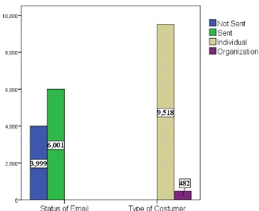
Fig. 1 Bar cart of Email Status and Costumer Type

The numbers of costumer for an individual was 9518 and the numbers of costumer for an organization was 482. About 3999 email was not sent to the costumers and 6001 email was sent to the costumers.

Fig. 2 Bar cart of Contract Answer and Costumer Defection

Contract Answer and Costumer Defection were the response variables. Fig. 2 showed that these variables were unbalanced. The proportion for costumer continues the contract was 0.008. It indicated that the variable of Contract Answer was unbalanced and rare event. The proportion for Costumer Defection was 0.6 and the proportion for non-defected was 0.4.

3.4 Classical bivariate binary logistic regression and Bayesian modeling

In this step, classical bivariate binary logistic regression and Bayesian modeling were applied in which 90% of data was used for modeling while 10 % of data was for testing data. This study used both small and large sample size. The number of small sample size was 200 samples and the number of large sample size was 10000 samples.

Tab. 2 Classical bivariate binary logistic regression and Bayesian modeling for a small sample size

Bayesian Estimates Using Gibbs Sampling Maximum Likelihood Estimates

Customer Defection

Contract

Answer Association

Customer Defection

Contract

Answer Association

Constants 2.0250000* -17.8400000 -0.5719000 0.0035408 -0.1766200 -24.0340000

Accumulation of Renewal -0.5527000* 1.8150000* -2.0900000 -0.0039161 -0.2896100 1.4144000

Price of Product 0.0000062 -0.0005852 0.8945000 0.0000497 0.0000063 0.0002382

Type of Costumer -0.1974000 -19.8900000 -0.0944400 0.0170110 -0.0773090 -9.5697000

Status of Email Delivery -1.3060000* 8.7690000 0.3139000 -0.0466380 -0.6392700 14.2700000

(9)

the model. Using Bayesian method, the variables having significant effect on the model were Accumulation of Renewal and Status of Email Delivery. By using classical method, the value of likelihood ratio test was 64.03, with a degree of freedom of 126 (64.03 < 153.198). It indicated the parameters were insignificant. However, this study ignored the finding.

Tab. 3 Classical bivariate binary logistic regression and Bayesian modeling for a large sample size

Bayesian Estimates Using Gibbs Sampling Maximum Likelihood Estimates

Customer Defection

Contract

Answer Association

Customer Defection

Contract

Answer Association

Constants 1.788000* -5.436000* -0.889800 0.016283* -0.187610* -7.543600*

Accumulation of Renewal -0.437300* -0.008472 1.789000 -0.00469* -0.026430* 0.218830*

Price of Product -0.000019 0.000020* -0.490900 0.000002* -0.000005* -0.000027*

Type of Costumer 0.093940 -28.150000* 0.143500 -0.00431* 0.073196* -11.64000*

Status of Email Delivery -0.941400* 0.906000* -0.662900 -0.03529* -0.470500* 2.558600*

Tab. 3 showed that all variables using large sample size were significant. The likelihood ratio test for

classical method was 1560.49, with a degree of freedom of 738. Using α = 5%, it can be concluded

that those parameters were significant (1560.49 > 802.310). It reaffirmed the findings of Lin, Lucas,

and Shmuali [10] that larger sample size will tend to reject H0 (for classical method).

3.5 Prediction results of classical bivariate binary logistic regression and Bayesian

The next step was comparing the prediction results of classical and Bayesian bivariate binary logistic regression. Logically, the higher is the percentage of validity, the better is the model. By using logit

function p x₁( )andp x2( ), prediction of the model was obtained.

Tab. 4 Classification of Customer Defection for a small sample size

Method Observed

Predicted _Overall

Percentage Data Customer

Defection=0

Customer Defection=1

Percentage Correct

Bayesian Customer Defection =0 41 35 53.947 70.556*

Training

Customer Defection =1 18 86 82.692

Classical Customer Defection =0 0 76 0 57.778

Customer Defection =1 0 104 100

Bayesian Customer Defection =0 6 2 75 90*

Testing

Classical Customer Defection =0 8 0 100 40

Tab. 5 Classification of Contract Answer for a small sample size

Method Observed

Predicted

Overall

Percentage Data

Contract Answer=0

Contract Answer=1

Percentage Correct

Bayesian Contract Answer=0 179 0 100 99.444

Training

Contract Answer=1 1 0 0

Classical Contract Answer=0 179 0 100 99.444

Testing

(10)

Tab. 6 Classification of Customer Defection for a larger sample size

Method Observed Predicted Overall

Defection=0

Percentage Correct

Bayesian Customer Defection =0 1826 1774 50.722 66.889*

Training

Classical Customer Defection =0 2678 922 74.389 61.433

Tab. 6 (Connection)

Method Observed

Predicted _Overall

Defection=0

Percentage Correct

Bayesian Customer Defection =0 203 197 50.75 69.200*

Testing

Classical Customer Defection =0 286 114 71.5 61.433

Tab. 7 Classification of Contract Answer for a larger sample size

Method Observed

Predicted

Overall

Percentage Data

Contract Answer=0

Contract Answer=1

Percentage Correct

Training

Testing

Based on Tab. 4 and Tab. 6, it was revealed that the appropriate method for classification of Customer Defection for small size sample and classification of Customer Defection for larger sample size is Bayesian method. This method had higher overall percentage than classical method. Tab. 5 and Tab. 7 showed that both of methods had the same overall percentage. Both of Tables were the classification of Contract Answer for small and large sample size. The variable Contract Answer was a rare event, so these methods were too difficult to predict the particular case.

5.

Conclusion

Based on the analysis and discussion, it can be concluded that the variables that affected Customer Defections and Contract Answer were Accumulation of Renewal, Price of Product, Type of Costumer, and Status of Email Delivery. These variables were significant evidenced by 10000 samples simulation in the model. The size of the sample used in the study affected the performance of the

model. For the classical approach, larger sample size had propensity to reject H0. Based on the

(11)

References

[1] K. Kanamori, M. Okada, H. Ohwada, and N. Prasasti. Customer Lifetime Value and Defection

Possibility Prediction Model Using Machine Learning: An Application to a Cloud-based

Software Company. Lecture Notes in Customer Science, 8398, 2013.

[2] N.P. Martono and H. Ohwada. Applicability of Machine Learning Techniques in Predicting

Customer Defection. In: International Symposium on Technology Management and Emerging

Technologies (ISTMET 2014), 2014.

[3] N. P. Martono. Customer Lifetime Value and Defection PossibilityPrediction Model Using

Machine Learning. Thesis, Department of Engineering of Industrial Administration, Tokyo University of Science, 2014.

[4] A. Asfihani. Prediksi Pembelotan Konsumen Software Antivirus ‘X’ dengan Binary Logistic

Regression dan Logistic Regression Ensembels. Final Project, Department of Statistics, Sepuluh Nopember Institute of Technology, 2015.

[5] P. McCullagh and J.A. Nelder. Generalized Linier Models (second edition). London: Chapman

and Hall, 1989.

[6] G. Ali, M. Darda, and Holmquist. Modelling of African Farm Dynamics Using Bivariate

Binary Logistic Regression in WinBUGS. Master Thesis, Department of Statistics, Lund University, 2009.

[7] Gary, King, and L. Zeng. Logistic Regression in Rare Events Data. Political Analysis,

9:2:137-163, 2001.

[8] R. L. Schaefer. Bias Correction in Maximum Likelihood Logistic Regression. Statistics in

Medicine, 2:71-78, 1983.

[9] M. Lin, H.C.Jr. Lucas, and G. Shmueli. Too Big to Fail: Large Samples and The P-Value

Problem. INFORMS, pp 1-12 ISSN 1526-5536, 2013.

[10] W. DuMouchel. Multivariate Bayesian Logistic Regression for Analysis of Clinical Study

Safety Issues. Statistical Science, Vol. 27, No. 3, pp 319-339, 2012.

[11] L. Briollais, R. I. Chowdhury, and M. A. Islam. A Bivariate Binary Model for Testing

Dependence in Outcomes. Bulletin of The Malaysian Mathematical Sciences Society, Vol. 35,

No. 4, pp 845-858, 2012.

[12] J.R. Dale. Global Cross-Ratio Models for Bivariate, Discrete, Ordered Response. Biometrics,

42, 909-917, 1986.

[13] J. Palmgren. Regression Models for Bivariate Binary Responses. Technical Reporty 101.

Departement of Biostatistics, School of Public Health and Community Medicine, Seatle, 1989.

[14] L. Cessie and R.L. Houwelingen. Logistic Regression for Correlated Binary Data, Applied

Statistic, 42, 95-108, 1994.

[15] B. P. Carlin and S. Chib. Bayesian Model via Markov Chain Monte Carlo Methods. Journal

Royal Statistical Society, 57, No.3, pp 473-484, 1995.

[16] S. Astutik, N. Iriawan, and D. D. Prastyo. Markov Chain Monte Carlo- Based Approaches for

Modeling the Spatial Survival with Conditional Autoregresive (CAR) Frailty. Journal of