Application HEC-HMS to Predict Hydrograph
(Case Study in Lebak Petal Sub Basin)
ESTRI RAHAJENG
MSc. In Information Technology for Natural Resources Management
Bogor Agricultural University, Indonesia
ABSTRACT
A hydrograph is a graph showing changes in the discharge of a river over a period of time. The main factors that influence hydrograph are imperviousness and curve number. Imperviousness is a very useful indicator which to measure the impact of land development on aquatic systems. The value of imperviousness is defined as the sum of roads, parking lots, sidewalks, rooftops, and other impermeable surfaces of the urban landscapes. The curve number is used to determine the amount of precipitation excess that results from a rainfall event over the basin. The purpose of this study is to predict unit hydrograph due to imperviousness and curve number changes.
Based on the result, increasing impervious areas lead to reduce infiltration and thereby increased surface runoff within catchments. It makes an effort to volume and peak discharge. From these values make an effort to time of peak discharge. The bigger value of imperviousness and curve number make time of peak early. The bigger value of imperviousness and curve number, make bigger value of peak discharge and volume. It means that imperviousness correlates highly with changes in hydrological indicators time to peak, peak discharge and volume. The outlet value indicates the amount of water flowing to the main channel. The bigger value of imperviousness and curve number make the bigger value of discharge.
Keyword :hydrograph, imperviousness, curve number
I.
Introduction
1.1 Background
A hydrograph is a graph showing changes in the discharge of a river over a period of time.
It can also refer
to a graph showing the volume of water reaching a
particular outfall, or location in a sewerage network,
related to time. Hydrographs are commonly used in the
design of sewerage, more specifically, the design of
surface water sewerage systems and combined systems.
The main factors that influence hydrograph are imperviousness and curve number.Imperviousness is a very useful indicator which to measure the impact of land development on aquatic systems. The value of imperviousness is defined as the sum of roads,
parking lots, sidewalks, rooftops, and other impermeable surfaces of the urban landscapes. Imperviousness is composed of two primary components: the rooftops under which we live, work and shop; the transport system (roads, driveways and parking lots) that we use to get one roof to another.
The curve number is an index developed by the Soil Conservation Service (SCS), now called the Natural Resource Conservation Service (NRCS), to represent the potential for storm water runoff within a drainage area. In calculating the quantity of runoff from a drainage basin, the curve number is used to determine the amount of precipitation excess that results from a rainfall event over the basin.
1.2 The Purpose
The purpose of this study is to predict unit hydrograph due to imperviousness and curve number changes
II.
Materials and Methods
2.1 Area Boundary
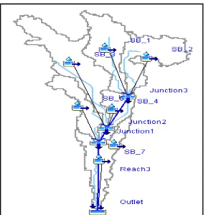
The study area is a part of the Lebak Petal sub basin in Musi Watershed. The geographic location of this study area is around 103° 34' 12" - 105° 0' 36" BT and 02° 58' 12" - 04° 59' 24". Based on the study of watershed management priority in 2006, the sub basin is the second priority sub basin. The study area is shown in figure 1.
2.2 Area Characteristics
The sub basin has 79.396,938 Ha areas. It consists of seven purposes of land use namely housing, local plantation, irrigated-paddy field, dry land, small lake, plantation estate and forest. Table 1 shows land use study area in Ha, the precentage of landuse purposes is dry land (71.45%), irrigated-paddy field (12.17%), local plantation (9.53%), plantation estate (3.24%), housing (1.75%), small lake (1.27%) and forest (0,59%).
Table 1. Land use purposes in study area
2.3 Data Preparation
The data that used to this study are:
1. Digital Elevation Model (DEM) of The Komering Sub Basin, can be obtained from www.cgiar.com (free download)
2. Soil Type Data of The Komering Sub Basin, can be obtained from Musi Watershed Management Agency, Ministry of Forest, 2009
3. Land Use Data of The Komering Sub Basin, can be obtained from Musi Watershed Management Agency, Ministry of Forest, 2009
2.4 Developing HEC-HMS model
2.4.1Preprocess the Terrain Model Open a new empty ArcMap project.
Add the Arc Hydro Tools toolbox to ArcToolbox. Load the Arc Hydro and HEC-GeoHMS toolbars. Load the terrain data.
Save the project.
Perform drainage analysis by processing the terrain using the 8-pour point approach.
Extract project specific data. 2.4.2Basin Processing
Revise subbasin delineation.
Extract physical characteristics of streams and subbasins.
Develop hydrologic parameters.
Develop HMS inputs. 2.4.3Hydrologic Modeling System
Setup an HMS model with inputs from HEC-GeoHMS.
The basin model in this modeling is generated from terrain processing and basin processing from HEC-GeoHMS embedded to ArcGIS 9.3.
2.4.1 Simulation by existing data (Musi).
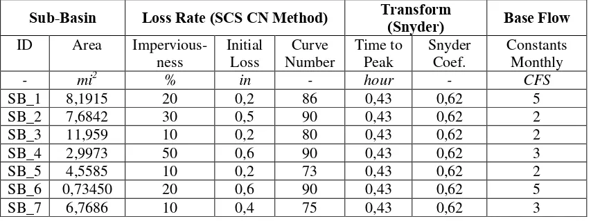
Data for each sub-basin are listed in table 2. The data include the sub-basin area, percent of imperviousness, and values of parameters that define losses, the runoff transform and base flow. Routing criteria for the basin reaches are listed in table 3.
Table 3. Routing Criteria
From To Method
Sub-Local plantation 7.563,405
Irrigated-paddy field 9.659,486
Dry land 56.735,238
Plantation estate 2.576,515
Small lake 1.007,138
Forest 467,189
Total Area 79.396,938
Figure 2. Basin Model in HEC-HMS
Rain gage data is to be distributed in time using temporal pattern of incremental rain fall, data from precipitation gage station are listed in table 4.
Table 4. Precipitation gage data (Jan 2-3, 2008)
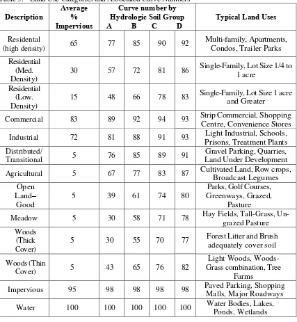
The changing of imperviousness and curve number to this practical report is based on table 5. Table 5 presents an example of typical land use categories used for hydrologic analysis, along with corresponding curve numbers for each land use-soil group combination. The land use categories shown in Table 5 were derived from the standard categories typically used for hydrologic analysis using the SCS methodology (SCS, 1986 in Marry C. Halley et. al, 2010).
Hydrologic Soil Group:
A = Soils having high infiltration rates, even when thoroughly wetted and consisting chiefly of deep, well to excessively-drained sands or gravels. These soils have a high rate of water transmission.
B = Soils having moderate infiltration rates when thoroughly wetted and consisting chiefly of moderately deep to deep, moderately fine to moderately coarse textures. These soils have a moderate rate of water transmission.
C = Soils having slow infiltration rates when thoroughly wetted and consisting chiefly of soils with a layer that impedes downward movement of water, or soils with moderately fine to fine texture. These soils have a slow rate of water transmission.
D = Soils having very slow infiltration rates when thoroughly wetted and consisting chiefly of clay soils with a high swelling potential, soils with a permanent high water table, soils with a clay pan or clay layer at or near the surface, and shallow soils over nearly impervious material. These soils have a very slow rate of water transmission.
III. Result and Discussion
3.1Global Summary Results
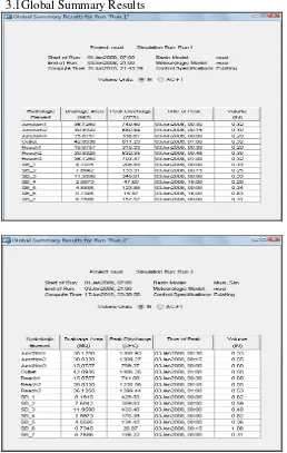
In fig 3. the changing of imperviousness and curve number to the sub basin area make some efforts to junction, reach and sub basin itself. Increasing impervious areas lead to reduce infiltration and thereby increased surface runoff within catchments. It makes an effort to volume and peak discharge. From these values make an effort to time of peak discharge. The bigger value of imperviousness and curve number make time of peak early. The bigger value of imperviousness and curve number, make bigger value of peak discharge and volume.
It means that imperviousness correlates highly with changes in hydrological indicators time to peak, peak discharge and volume. As illustration, because there is no opportunity for plants to absorb the moisture that falls on pavement, a much larger volume of storm water drains into streams that flows from urban areas. This large quantity of water reaches streams too quickly, flowing across roads and
through pipes that do not offer the resistance to surface flow that natural vegetation of meadow and forests.
3.2 Time-Series Results
In fig 4. time series data consist of loss, excess, direct flow, base flow and total flow. In this case, only using SB_1 represents the trend of these values. In Musi result, direct flow was started on 2 January 2008 at 09.15 and had value 0.708 cfs. The excess value was still zero and the loss value was 0.005 in. In Musi_Sim result, direct flow was started on 2 January 2008 at 09.15 and had value 2,831 cfs. The excess value was 0,001 in and the loss was 0.004 in.
For the total flow, Musi_sim has bigger value than Musi result. It relate to the changing of imperviousness and curve number in Musi_sim. The bigger value of imperviousness and curve number make the bigger value of total flow. Total flow is the result of summary from direct flow and base flow.
Figure 3. Global Summary Results for Musi and Musi_Sim
Figure 4. Time-Series Results for SB_1 in Musi and Musi_Sim
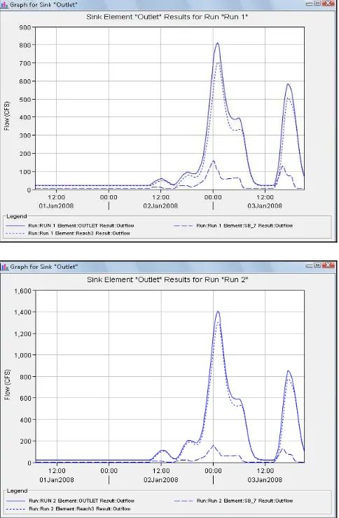
3.3 Outlet Discharge
In fig 5. the graphs of outlet discharge consist of outlet, reach3 and SB_7 outflow graph. Due to the outlet is related to these 3 components directly. The outlet value indicates the amount of water flowing to the main channel. The outlet value of Musi_Sim results is bigger than Musi results; it means that the imperviousness and curve number make significant different value between both. These conditions of
results are the same trends with Reach3 results. For SB_7, the outlet value in Musi_Sim is same with Musi since SB_7 isn’t related to the other component of basin. Selamat
4 Conclusion
Changing in land use/land cover will affected to the curve number and imperviousness value. The small value of curve number will give low water discharge value, and the big value of curve number will produce high water discharge value.
The water discharge value indicates run off value for these catchment area. The run off value closely tracks percent impervious cover. Increasing impervious coverage makes increasing imperviousness value.
5. Acknowledgement
REFERENCES
HEC Geo-HMS Tutorial. ESRI Production.
Mary C. Halley P.E. , Suzanne O. White, and Edwin W. Watkins P.E. 2010. ArcViewGIS Extension for
Estimating Curve Numbers.
www.proceeding.esri.com.html
Pawitan. H, Trihono Kadri. 2010. Problem Set. ITM 616 Hydrologic Modeling. Bogor
www.wikipedia.org/wiki/imperviousness
Table 2. Sub-basin characteristics / Parameter (Musi)
Table 5. Land Use Categories and Associated Curve Numbers
Description
Sub-Basin Loss Rate (SCS CN Method) Transform
(Snyder) Base Flow
Table 5. Sub-basin characteristics/parameter (Changing/simulation data)
Sub-Basin Loss Rate (SCS CN Method) Transform
(Snyder) Base Flow
ID Area Impervious-ness
Initial Loss
Curve Number
Time to Peak
Snyder Coef.
Constants Monthly
- mi2 % in - hour - CFS
SB_1 8,1915 20 0,2 86 0,43 0,62 5
SB_2 7,6842 30 0,5 90 0,43 0,62 2
SB_3 11,959 10 0,2 80 0,43 0,62 2
SB_4 2,9973 50 0,6 90 0,43 0,62 3
SB_5 4,5585 10 0,2 73 0,43 0,62 2
SB_6 0,73450 20 0,6 90 0,43 0,62 5