DOI: 10.12928/TELKOMNIKA.v14i1.2400 294
Detection and Prediction of Peatland Cover Changes
Using Support Vector Machine and Markov Chain
Model
Ulfa Khaira*1, Imas Sukaesih Sitanggang2, Lailan Syaufina3 1,2
Department of Computer Science, Faculty of Natural Science and Mathematics, Bogor Agricultural University, Indonesia
3
Department of Silviculture, Faculty of Forestry, Bogor Agricultural University, Indonesia *e-mail: [email protected]
Abstract
Detection and prediction of peatland cover changes should be conducted due to high rate deforestation in Indonesia. In this work we applied Support Vector Machine (SVM) and Markov Chain Model on multitemporal satellite data to generate the correspondings detection and prediction. The study area is located in the Rokan Hilir district, Riau Province. SVM classification technique used to extract information from satellite data for the years 2000, 2004, 2006, 2009 and 2013. The Markov Chain Model was used to predict future peatland cover. The SVM classification result showed that the mean Kappa coefficient of peatland cover classification is 0.97. Between years 2000 and 2013, the wide of non vegetation areas and sparse vegetation areas have increased up to 307% and 22%, respectively. While the wide of dense vegetation areas have decreased up to 61%. We found that a 3 years interval used in the Markov Chain Model leads to more accurate results for predicting peatland cover changes.
Keywords: change detection, markov chain model, multitemporal, peatland, support vector machine.
Copyright © 2016 Universitas Ahmad Dahlan. All rights reserved.
1. Introduction
Forest cover as one indicator of forest condition is continuesly decreasing due to human exploitation. Indonesia is the fourth country with the world's largest peatland with 19.3 million ha of peatland. At the end of 2013, there are about nine million ha area still covered with natural forests. In 2009-2013 there are approximately 1.1 million ha of natural forests on peatlands had lost and those are more than a quarter of the total area of natural forest cover loss throughout Indonesia. The largest natural forests cover loss in peatland during the period 2009-2013 is in Riau Province in the amount of 450 thousand ha [1].
Peatland is one area that should be protected because it can keep carbon (C) in huge numbers. Peatland has high water retention power so it can be support the hydrology of surrounding area, peatland can tie up the carbon thus contribute to reduce greenhouse effect in the atmosphere. The amount of carbon stocks depend on the depth of the peat. If the peat forest isharvested and the land is drained, the carbon in it will easily oxidized into CO2 gas so that the changes will disrupt all the peatland ecosystem function [2].
sensing technology has many important roles, like reduction of survey time, latest map availability, and digital image classification (pixels).
A wide variety of digital changes detection algorithms have been developed over the last two decades to changes in different land covers. Support vector machine (SVM) is a group of supervised classification algorithms that have been used recently in the remote sensing field [4]. Many researchers in this field have found that the higher accuracy is produced by SVM than other process of classification like Maximum Likelihood (MLC) dan Artificial Neural Network (ANN) [5-8]. This research will be carried out peat land cover classification using SVM based on the value of the digital number (DN). Land cover changes detection can be done by comparing the results of land cover classification of two satellite imagery in the same area and were taken at different times.
After finding out how much the changes in land cover, we can make predictions about the trend of land cover changes in the future. The model which is used commonlyin predicting land cover changes is the Markov chain model. The use of this model has been used to study vegetation dynamics and land cover changes in different ecological zones [9]. Results of predicting land cover changes by this model, however, depend on the time interval from which the matrix probability is derived. The use of Markov chain models for predicting trends of urbanization in Jordan showed good results with predictions and actual suitability index of 0.982 for satellite imagery with nine years interval [10].
This research applied the SVM with RBF kernel for land cover classification and the Markov chain model to build land cover change prediction with 3, 6, and 9 years interval, this study also evaluated the effect of time-interval on predicting land cover changes so that the time interval of satellite imagery with the highest accuracy of prediction will be recommended for predicting future land cover. The aims of this study are to assess the peatland cover changes using multi-temporal remotely sensed data and to predict the amount of peatland cover in the future inRokan Hilir district Riau province.
2. Research Method
2.1. Study Area and Datasets
The study area is Rokan Hilir District in Riau Province, Indonesia. It covers an area of 8,881.59 km2. The geographical location of the district is 100o 17’ – 101o 21’ East Longitude and 1o 14’ – 2o 45’ North Latitude. Rokan Hilir is one of districts in Riau that had 454,000 ha of peatlands in 2002 [11]. This research focus on peatland with more than 4 meter deep at Rokan Hilir District.
The multi-temporal dataset consists of three Landsat 5 TM images patch 127, row 59 and two images from Landsat 7 ETM+ (Table 1). These images were acquired freely from the official website of United States Geological Survey (USGS, http://earthexplorer.usgs.gov). The images included the shortwave infrared (SWIR), the near infrared (NIR), and the visible (band 3) with 30 m spatial resolution for TM and ETM+ images. The spatial data such as administrative boundaries and peatland characteristics were obtained from Ministry of Forestry Republic of Indonesia.
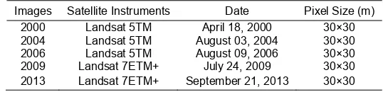
Table 1. Landsat Scenes Used
Images Satellite Instruments Date Pixel Size (m) 2000 Landsat 5TM April 18, 2000 30×30 2004 Landsat 5TM August 03, 2004 30×30 2006 Landsat 5TM August 09, 2006 30×30 2009 Landsat 7ETM+ July 24, 2009 30×30 2013 Landsat 7ETM+ September 21, 2013 30×30
2.2. Image Preprocessing
datum and ellipsoid. Radiometric correction is used to remove sensor or atmospheric noise to more accurately represent ground conditions. On May 31, 2003 the Scan Line Corrector (SLC) in the ETM+ instrument failed. All images were taken after that date have gap, approximately 22% of the data in a Landsat 7 scene is missing. This gap filling process can be done using Frame and Fill software which is open source software from NASA. Creating a composite image from Landsat Imagery by combining band 5 (SWIR), band 4 (NIR), and band 3 (red). The 5, 4, 3 band combination refers to the standard of the Ministry of Forestry for forest and vegetation analysis. Figure 1 shows the result of images preprocessing, the image has dimensions of 2682x3599 pixels.
Figure 1. The result of images preprocessing
2.3. Support Vector Machine Classification
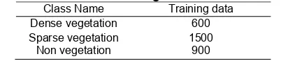
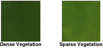
The support vector machine supervised classification was applied to identify the class associated with each pixel. There are three steps involved: training, running classification algorithm, and accuracy asessment. For supervised classification, training sides are needed. Classification involves labelling the pixels as belonging to particular spectral (and thus information) classes using the spectral data available. Supervised classification methods are trained on labeled data. Sufficient training samples for each spectral class must be available to allow reasonable estimates of the elements of the mean vector and the covariance matrix to be determined. As the number of bands increases the number of training data classification is increased too. In usual the minimum number of training data for each class is 10N, where N is the number of bands [12].This means that for a three band Landsat image the size of the training sample required minimum 30 pixels. Due to the coarse resolution of the data, three classes were considered in the analysis: dense vegetation (dark green), sparse vegetation (yellow-green), and non vegetation (brown) (Figure 2). The details about the number of training pixels are shown in Table 2.
Table 2. Number of Training Data for Classification Class Name Training data
Dense vegetation 600 Sparse vegetation 1500
Non vegetation 900
SVMs function by nonlinearly projecting the training data in the input space to a feature space of higher (infinite) dimension by use of a kernel function. In this study, the radial basis function (RBF) kernel method was chosen. RBF kernel requires setting of two parameters, the kernel width γ and the cost parameter C to quantify the penalty of misclassification errors. Implementation of the training and testing SVM model process using LIBSVM in package e1071, the e1071 package was the first implementation of SVM in R language program. Little information exists in the literature on how to identify these parameters, therefore in this study we use grid-search over specified parameter ranges. It returns the best values to use for the parameters γ and C. The ranges of γ parameter is 10-6-10-1 and 10-1-101 for C parameter.
Dense Vegetation Sparse Vegetation Non Vegetation
Figure 2. The example of land cover types
2.4. Accuracy Assesment
Accuracy asessment was performed to evaluated the results of SVM classification. Standard confusion matrix was used to perform the accuracy, the reference data were divided into training and testing sample data and used to asses classification accuracies. Two measures of accuracy were tested, namely overall accuracy and Kappa coefficient. The error matrix was used to show the accuracy of the classification result by comparing the classification result with ground truth point [16].
2.5. Changes Detection
Change detection statisics were used to compile a detailed tabulation of changes between two classification images [17]. A multi-date post-classification comparison change detection algorithm was used to determine changes in land cover in four intervals, 2000-2006, 2006-2009, 2000-2009, and 2000-2013. This technique is widely used because it is easy to understand and requires final classification maps with the highest accuracy possible to be compared pixel-by-pixel. The post-classification approach provides “from-to” change information in order to identify the transformations among the land cover classes and the kind of transformation that have occured can be easily calculated [16].
2.6. Modeling of Land Cover Changes
In this study, land cover change detection was divided by two conditions, past and future time. Past condition were analyzed by using SVM supervised classification and post-classification method. Meanwhile, the future condition was analyzed by a Markov chain method based on past land covers.Markov chain were used to gain the percentage and probability for each type of land cover convert to other land cover type. A first-order Markov chain model is a model of such a system in which probability distribution over next state was assumed to only depend on current state (not on previous ones) [18]. A first-order Markov model was used to represent the land cover change for diffrent time intervals. Future land cover was predicted by multiplying the state vector (initial land cover) at a given time (Vinitial) by the transition matrix [Pij] during a time interval t to yield the new state vector (Vinitial+t) or expected proportion of land cover
after t yeras after the initial state as follows [10]:
Vinitial × [Pij]t = Vinitial+t
intervals. This procedure was carried out for the combinations 2000-2006, 2006-2009, and 2000-2009. The aim was to evaluate the accuracy of prediction using 3, 6, and 9 years interval based on the rate of land cover change during 2000 to 2009. The Markov model was used to predict future land cover using the time interval with the highest accuracy of prediction to predict future land cover. There are two statistical method to evaluate the accuracy of prediction, the RMSE and the index of agreement (D). The RMSE and D were computed as follows [19].
RMSE = ∑ .
D= 1 - ∑
∑ ′ ′
N is the number of land cover classes, P is the predicted class and O is the observed class,
′ dan ′ , is the mean of the observed values of land cover. The lower
the RMSE is the better agreement. A value of 1 for D means a complete agreement between predicted and actual land cover.
3. Results and Analysis
3.1. Image Classification Using SVM
Supervised image classifications were applied to the 2000, 2004, 2006, 2009, and 2013 images using SVM classification technique. The number of pixels in the training dataset was 2000 and the number of pixels in the testing dataset was 1000. In this sudy, we did SVM classification for three classes. These classes are dense vegetation, sparse vegetation, and non vegetation. Through in using SVM some parameters had to be considered, the RBF kernel method was chosen. In order to use RBF kernel, the two γ and C must be put. We use grid-search to obtain the best parameter of γ and C . Through the process of grid-serach, the best values for γ and C parameters were 0.1 and 10 respectively. After we have got the best values of paramters, we must do SVM classification method on Landsat images. Standard confusion matrix was used to perform the accuracy assesment of image classifications. For evaluating SVM accuracy, tetsing data have been used. The accuracy of the data for the years 2000, 2004, 2006, 2009, and 2013 was 95%, 99%, 100%, 99%, and 98% respectively. Similarly, the Kappa coefficient was 0.92, 0.98, 1, 0.99, and 0.98. The mean overall accuracy of classification was 98.2% and mean Kappa coefficient was 0.97. Based on standards quoted by Treitz and Rogan [20] land cover map accuracy should be more than 85% for land cover change detection study.
3.2. Land Cover Change Analysis
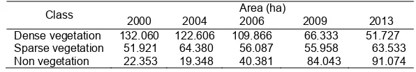
After applying the classification scheme on all five images the area of each class was determined as Table 3. The results show that there is an increment in non vegetation areas during the period of 2000 to 2013. On the other hand, the dense vegetation areas was decreased. The trend of change for non vegetation areas was different from the dense vegetation.
Table 3. Area of Land Cover Classes
Class 2000 2004 2006 2009 Area (ha) 2013
Dense vegetation 132.060 122.606 109.866 66.333 51.727 Sparse vegetation 51.921 64.380 56.087 55.958 63.533 Non vegetation 22.353 19.348 40.381 84.043 91.074
the major diagonal of the matrix. Table 4 shows important trends of land cover changes during 13 year period. In term of area, 56.373 ha of the dense vegetation and 23.711 ha of the sparse vegetation areas was changing into non vegetation areas. These result indicate that increase in non vegetation areas mainly came from conversion of the dense vegetation to the non vegetation during 13 year period.
Table 4. The Matrix of Area Land Cover Change between 2000 (rows) and 2013 (columns)
Year 2013
Dense vegetation 46.142 29.546 56.373 132.061 -80.335 -61 Sparse vegetation 4.942 23.269 23.711 51.922 +11.611 +22 Non vegetation 643 10.718 10.990 22.351 +68.723 +307 Total Area 51.727 63.533 91.074
3.3. Future Land Cover
Land use change is defined as a function of probability. The probability component of land use change is expressed in a matrix known as a transition probability matrix. Each class of land cover has different change probabilities between one of classes with another class. In order to construct the transition probability matrix, land cover maps were cross-tabulated to derive tables that represented transition matrices where the change of type i into type j was calculated. The set of all possible transition i-j, divided by the total area of type i in the initial state, Transition probabilities were expressed as a complete matrix of land cover classes, where the rows of the matrix sum to 100%, and the diagonal cells represent the unchange class. This matrix was used to calculate Pij by dividing the area of each row by the row’s total [10]. Table 5 showed the transition matrix between 2000 and 2009, in this matrix, for example, the probability of changing dense vegetation into other classes is 24% to sparse vegetation and 30% to non vegetation, while 46% of the dense vegetation remained unchage.
Table 5. The Matrix of Percentage Land Cover Change between 2000 (rows) and 2009 (columns)
Year 2009
Dense vegetation Sparse vegetation Non vegetation
Year 2000
Dense vegetation 46 24 30 Sparse vegetation 10 33 57 Non vegetation 2 32 66
Prediction for future land cover was based on the initial map of 2004 (Vinitial) using the
transition matrix of 9 years (2000-2009). The output land cover was predicted for year 2013. Similarly, The initial map of 2006 (Vinitial) using the transition matrix of 6 years (2000-2006), and
the transition matrix of 3 years (2006-2009) using the map of 2009 as the Vinitial . Results from land cover prediction showed variations in the future trends of land cover based on to the time interval from which the probability matrix was derived as Table 6. There are two statistical method to evaluate the accuracy of prediction, the RMSE and the index of agreement (D). A value of 1 for D means a complete agreement between predicted and actual land cover.
Table 6. The Actual and The Predicted Results (%) from The Markov Chain Model in 2013 Class Land Cover Prediction for 2013 According to the Time Interval (%)
Table 6 showed that the use of multi-temporal satellite imagery with 3 years interval would provide accurate results for predicting peatland cover changes.
In this study, we assumed continuous change of land cover following historical trends. To predict future land cover, we apply the transition matrix for the time interval with the maximum accuracy of the prediction. The transition parobability in the Markov chain model is assumed to be uniform. Result of land cover prediction showed that non vegetation areas would expand in the future and would reach 53% in year 2016. The increase of non vegetation areas in line with the increasingly unsustainable forest exploitation carried out by companies and individuals.
4. Conclusion
Three Landsat 5 TM and two Landsat 7 ETM images over a thirteen-year time period from 2000 to 2013 were used for examining land cover changes in Rokan Hilir district, Riau province, Indonesia by applying SVM classification and Markov chain model. The mean overall accuracy of classification was 98.2% and mean Kappa coefficient was 0.97. Between years 2000 and 2013, the wide of non vegetation areas and sparse vegetation areas have increased up to 307% and 22%, respectively, with the greatest increase occurring from 2006 to 2009. While the wide of dense vegetation areas have decreased up to 61%. The main overall change trend was the increase in non vegetation areas. Prediction of future land cover change by the Markov chain model showed that the use of multi-temporal atellite imagery with 3 years interval would provide accurate results for predicting peatland cover changes. Markov modelling showed that by 2016, the non vegetation areas would increased about 53%. The future land cover maps of this study area may be different from the actual land cover later, it can be caused by climate, governmental policy, and human disturbance that applied in the study area during the transition periods.
References
[1] Indonesia, Forest Watch, Global Forest Watch. The state of the forest: Indonesia. Bogor: Forest Watch Indonesia and Global Forest Watch. 2002.
[2] Agus F, Subiksa IGM. Lahan Gambut: Potensi untuk pertanian dan aspek lingkungan. Balai
Penelitian Tanah dan World Agroforestry Centre (ICRAF). Bogor. 2008.
[3] Du P, Liu S, Gamba P, Tan K, Xia J. Fusion of difference images for change detection over urban areas. IEEE journal. 2012; 5(4): 1076-1086.
[4] Kavzoglu T, Colkesen I. A Kernel Functions Analysis For Support Vector Machines For Land Cover
Classification. International Journal of Applied Earth Observation and Geoinformation. 2009; 11(5):
352-359.
[5] Mondal A, Kundu S, Chandniha SK, Shukla R, Mishra PK. Comparison Of Support Vector Machine
And Maximum Likelihood Classification Technique Using Satellite Imagery. International Journal of
Remote Sensing and GIS. 2012; 1(2): 116-123.
[6] Naguib AM, Elwahab A, Farag MA, Yahia MA, Ramadan HH. Comparative Study Between Support Vector Machines and Neural Networks for Lithological Discrimination Using Hyper spectral Data.
Egypt Journal of Remote Sensing and Space Science. 2009; 42(25): 27-24.
[7] Cheng L, Bao W. Remote sensing image classification based on optimized support vector machine.
TELKOMNIKA Indonesian Journal of Electrical Engineering. 2014; 12(2): 1037-1045.
[8] Yang N, Li S, Liu J, Bian F. Sensitivity of Support Vector Machine Classification to Various Training
Features. TELKOMNIKA Indonesian Journal of Electrical Engineering. 2014; 12(1): 286-291.
[9] Balzter H. Markov Chain Models For Vegetation Dynamics. Ecological Modelling. 2000; 126(2):
139-154.
[10] Al-Bakri JT, Duqqah M, Brewer T. Application Of Remote Sensing And GIS For Modelling And
Asssesment Of Land Use/Cover Change In Amman Jordan. Journal of Geographic Information
System. 2013; 5(5): 509-519.
[11] Wahyunto, Suryadiputra INN. Peatland Distribution in Sumatra and Kalimantan-explanation of its Data Sets Including Source of Information, Accuracy, Data Constraints and Gaps. Bogor: Wetlands International, Indonesia Programme. 2008.
[12] Davis SM, Landgrebe DA, Phillips TL, Swain PH, Hoffer, RM, Lindenlaub JC, Silva LF. Remote sensing: the quantitative approach. New York: McGraw-Hill International Book Co.1978.
[13] Huang C, Davis LS, Townshend JRG. An Assessment Of Support Vector Machines For Land Cover Classification. International Journal Of Remote Sensing. 2002; 23(4): 725-749.
Training Data Acquisition For SVM Classification. Remote Sensing of Environment. 2004; 93(1): 107-117.
[15] Anthony G, Gregg H, Tshilidzi M. Image Classification Using Svms: Against-One Vs
One-Against-All. Proccedings of the 28th Asian Conference on Remote Sensing. Kuala Lumpur. 2007; 2:
801-806.
[16] Yuan F, Sawaya KE, Loeffelholz BC, Bauer ME. Land Cover Classification And Change Analysis Of
The Twin Cities (Minnesota) Metropolitan Area By Multitemporal Landsat Remote Sensing. Remote
sensing of Environment. 2005; 98(2): 317-328.
[17] Al-Doski J, Mansor SB, Shafri HZM. Support vector machine classification to detect land cover
changes in Halabja City, Iraq. IEEE Business Engineering and Industrial Applications Colloquium
(BEIAC).Langkawi. 2013: 353-358.
[18] Guan D, Gao W, Watari K, Fukahori H. Land Use Change Of Kitakyushu Based On Landscape
Ecology And Markov Model. Journal of Geographical Sciences. 2008; 18(4): 455-468.
[19] Krause P, Boyle DP, Bäse F. Comparison of Different Efficiency Criteria for Hydrological Model
Assessment. Advances in Geosciences. 2005; 5: 89-97.