The use of analysis of covariance in the

(1)

J.

zyxwvutsrqponmlkjihgfedcbaZYXWVUTSRQPONMLKJIHGFEDCBA

Fish BioI.

zyxwvutsrqponmlkjihgfedcbaZYXWVUTSRQPONMLKJIHGFEDCBA

(1984)

24, 201-213

The use

of

analysis

of covariance in the back-calculation

of growth in fish

J. R.

BARTLETT,

P. F. RANDERSON,

R. WILLIAMS

AND

D. M. ELLIS*

Department of Applied Biology and *Department of Mathematics, UWIST,

King Edward VII Avenue, Cardiff (Accepted I 7 May 1983)

I. INTRODUCTION

Techniques for the back-calculation of the growth histories of fish populations have been developed since the beginning of this century. Notable among the early workers were Dahl ( 1909), Lea ( I 9 lo), Lee (1 9 12) and Monastyrsky ( 1930). Re- views of the subject are contained in Lee (1920), Graham (1 929), Lagler ( I 956), Hile (1970), Weatherley (1972) and Bagenal & Tesch (1978). The basic process remains unchanged from that used by Dahl and Lea and comprises three stages:

( 1) An indicator calcified structure such as a body scale, otolith, cleithrum or

cross-section of a bone is chosen. This should contain marks indicating yearly increments of growth providing a clear representation of the growth history of the structure and, by inference, of the fish.

(2) Data are collected, from a sample of fish, on body length and of indicator- structure size, e.g. scale radius along a particular axis, at the time of capture.

(3) A plot of body length against structure size is used to establish the form of the relationship. This may be through or not through the origin, curved, sig- moidal or a complex of different linear or curved relationships (Wooland & Jones,

1975).

This paper relates to the problems associated with the use of linear regression analysis when attempts are made to establish the body length : indicator-structure relationship. Linear regression analysis may be inadequate and produce inaccur- ate results for two reasons; first, it is an attempt to fit a straight line through the data regardless of the true form of the relationship and second, it does not allow for objective comparison between the fit of regression lines with alternative trans- formations of the same data. Carlander (1981) has noted that a sample of fish, taken at one time, contains a series of year classes and deviations from a linear or curved body length : indicator-structure relationship may arise unless regressions are calculated for each age class.

These problems are illustrated by considering a case in which a plot of body length and indicator-structure data shows a slightly curved trend (Fig. 1).

Although linear regression analysis of these data may show a significant relationship, the fitted line would not accurately follow the curve shown by the data. In many cases analysis of the body length : indicator-structure relationship would

20 I

(2)

202

zyxwvutsrqponmlkjihgfedcbaZYXWVUTSRQPONMLKJIHGFEDCBA

J . R . B A R T L E T T

E T A L .

I

I I I

25

50

75 100

0

Scale radius (arbitrary optical unlts)

FIG. 1. Relationship between body length and scale-radius from a sample of81 roach, Rufilus ru/ilus.

zyxwvutsrqponmlkjihgfedcbaZYXWVUTSRQPONMLKJIHGFEDCBA

showing regression lines fitted to the untransformed data (dashed line) and to the age-group

means of the logarithmically transformed data. 0: 8 I individual fish;

zyxwvutsrqponmlkjihgfedcbaZYXWVUTSRQPONMLKJIHGFEDCBA

0: means for age groups

1-9.

end at this point and back-calculation would be performed using one of the expressions (I), (2) or ( 3 ) .

s n

L,, =-L ( I ) Lea(1910)

S

(2) Lee (1 920)

L, = a+b S, ( 3 ) Fraser (1 9 16) where L= length of fish when sample was obtained; L,= body length at the time

of formation of the nth annulus; S,=length of indicator structure at the nth annulus; S= length of indicator structure (e.g. total scale radius) when sample was obtained; and a and b are parameters of the regression line.

The linear regression method will not indicate whether a transformation is necessary and, if so, the type. Transformation may be needed to allow for a curved relationship (Fig. l), for non-constant variation about the relationship, or for both.

(3)

B A C K - C A L C U L A T I O N OF

zyxwvutsrqponmlkjihgfedcbaZYXWVUTSRQPONMLKJIHGFEDCBA

GROWTH

203

Unfortunately, it would not then be possible for an investigator to determine which of the regressions offered the more accurate description of the true body :

indicator relationship and hence which of the two sets of back calculated results was the more realistic. If ANOVA of the two regressions both show a significant F-ratio, it is not then possible to say that one is the more significant and likely to be reproducible in further samples. Therefore the choice of expression for use

in back-calculation could only be made on an arbitrary basis.

zyxwvutsrqponmlkjihgfedcbaZYXWVUTSRQPONMLKJIHGFEDCBA

11. THE ANALYSIS OF COVARIANCE

It is in situations such as this that another statistical technique, analysis of covariance, may hold an advantage over these conventional methods. Analysis of covariance can be used to derive a clear description of the trends in the data by comparing the relationship between body length and indicator-structure size in three ways. Regression analysis is performed first, on the data as a whole, second on groups of the data divided according to a third variable (covariate), the age of fish at capture, and finally on the mean values of body length and indicator- structure size for each age group.

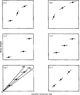
The analysis of covariance distinguishes four models dependent upon the source of the significant F-ratio. These alternatives are illustrated in Fig. 2 and are summarized as follows:

( 1 ) The slopes of the lines fitted through the separate subsets of the data differ significantly from one another [Fig. 2(a)]. Further investigation may indicate a pattern in this variation as in Fig. 2(b). An overall regression line should not be fitted to the data as they stand, neither should back-calculation be performed. However, back-calculation may be possible following transformation of the data. For instance if the data showed the curved trend of Fig. 2(b), then transformation to logarithms might, on subsequent analysis of covariance, demonstrate an overall linear trend.

(2) The slopes of the lines through individual age groups do not differ significantly but their mean values show a significant deviation from a straight line [Fig. 2(c)]. In this case the lines in the separate groups are parallel. Back-calculation’ cannot be performed on the data in their present form.

(4)

204 J . R . B A R T L E T T

zyxwvutsrqponmlkjihgfedcbaZYXWVUTSRQPONMLKJIHGFEDCBA

E T A L .

- I

-

Indicator-structure

size

FIG. 2 . An illustration of the possible models distinguished by analysis of covariance.+: Mean value and regression line through the data of one age group. (See text for an explanation of lines

OB, OM and OC).

zyxwvutsrqponmlkjihgfedcbaZYXWVUTSRQPONMLKJIHGFEDCBA

common intercept on the ordinate (Fraser, 19 16) then back-calculation could be

performed using expression (2). This expression derives only the intercept term,

a,. from the line through the means. Its other terms comprise the individual’s

own body length : indicator-structure relationship.

These assumptions are similar to those developed by Hile (1941) in work on

the rock bass, Ambloplites

zyxwvutsrqponmlkjihgfedcbaZYXWVUTSRQPONMLKJIHGFEDCBA

rupestris. Having fitted a regression line to the body length : scale radius relationship, Hile found that some fish had scales which were [image:4.468.99.368.68.387.2]

(5)

BACK -CA LCU LATlON OF GROWTH

zyxwvutsrqponmlkjihgfedcbaZYXWVUTSRQPONMLKJIHGFEDCBA

205

where Ao=observed radius of the nth annulus; Ar=expected (or corrected) radius of the nth annulus; S,=observed scale radius; &,=expected scale radius of a fish of given body length.

Back-calculation was then carried out using the equation describing the sample regression line. Whereas the assumptions involved in the use of expression (2)

and in Hile’s correction method

zyxwvutsrqponmlkjihgfedcbaZYXWVUTSRQPONMLKJIHGFEDCBA

(4) are identical, the former has the advantage in being the more direct calculation.

(4) Where no other source in an analysis of covariance gives a significant F-ratio then that due to the fit of the overall line should do so [Fig. 2(0]. Back- calculation could then be performed using the equation for the line:

L, =

a,+b, S, ( 5 )

a, =

L,

- b,

S,

₍₆₎

where a,= intercept on ordinate (body length), i.e. and b,= slope of the overall regression line.

111. THE METHOD OF ANALYSIS OF COVARIANCE

The steps in the analysis of covariance are given as an aid to those unfamiliar with the technique. After the basic sums of squares and products have been obtained from each age group of raw data, calculation of the covariance statistics is not lengthy.

The first step in an analysis of covariance is to separate the sample data into subsets according to the age of the fish at capture. The analysis will then examine the variation of the body length : indicator-size relationship that exists between successively older groups of fish.

Regression analyses of body length ( y ) on indicator-structure size (x) are then performed on the data of each subset. The regression statistics are then tabulated as:

2x9

ZY>

29,

zx2, ~ X Y , Sj(x,x),

zyxwvutsrqponmlkjihgfedcbaZYXWVUTSRQPONMLKJIHGFEDCBA

sj(YFY)v), Si(x,Y)

where

S,(x,y) = individual age group’s corrected sum of products.

CXCY

Si(x,Y)

= ~ X Y - ___

n

(6)

206

J .

R. B A R T L E T T

E T A L .

These statistics are then summed across all age groups and the following derived from them.

where N=total number of fish in the sample. Sl(x,x) and S,(x,y) are then found similarly and Al as:

(St ( X > Y ) Y

zyxwvutsrqponmlkjihgfedcbaZYXWVUTSRQPONMLKJIHGFEDCBA

s,

( X J )

At

= S,(Y,Y)-

S,(x,x) is calculated as:

S,(X,X) = ~ S i ( X , X )

Sa(x,y) and S,(y,y) are found similarly. Then Aa is calculated as:

(9)

Although not directly required in the analysis the slopes of certain lines can be obtained from the above statistics. For instance the slope of the regression line through a single age group’s results, b j is:

If it is decided that parallel lines may be used in the subsets of data the common slope, b,, is calculated as:

(7)

BACK-CALCULATION OF G R O W T H

207

TABLE I. Compilation of the analysis of covariance result table

Source Degrees of Sums of squares square Mean P-ratio

*

free do m

Total

N - 1

&CV3Y 1 ss/df ms/rms

Due to the overall

line

(h,)

I

Difference of I At-

A m - Aa ss/df ms/rms Fig. 2(d)

Deviation of the

B, and h,

ss/df ms/rms Fig. 2(c)

ss/df ms/rms Fig. 2(a)

ss/df - -

means from a K - 2

zyxwvutsrqponmlkjihgfedcbaZYXWVUTSRQPONMLKJIHGFEDCBA

Am

Between slopes (hi) K - 1 A0 - A,

Residual _{N - 2 K} A,

straight line (b,)

Where N=number of fish in the sample; K=number of age groups present in the sample; ss=sum

*Appropriate model if the F ratio is significant.

of squares; df= degrees of freedom; rns = mean square; rms = residual rns.

If all results may be fitted by a single regression, the line has the slope b,:

SSXSY)

b, = ___

zyxwvutsrqponmlkjihgfedcbaZYXWVUTSRQPONMLKJIHGFEDCBA

S/(XJ)

The results table of the analysis of covariance is then compiled in the form shown in Table I.

As in a table of ANOVA, each mean square term is calculated as the ratio of the sum of squares by the appropriate degrees of freedom. Analysis of covariance is then completed by calculation of the ratio of each mean square value to the residual mean square. The models are tested in the order 2(a), 2(c), 2(d) 2(f) using the F-ratios indicated in Table I.

IV. AN EXAMPLE OF THE USE OF ANALYSIS OF COVARIANCE IN Body length, scale radii and annular radii were recorded on a sample of 81

roach, Rutilus rutilus. Linear regression analysis of data for body length

zyxwvutsrqponmlkjihgfedcbaZYXWVUTSRQPONMLKJIHGFEDCBA

01)

on scale radius (x) gave the following results:

BACK-CALCULATION

Slope of the regression line = b ' = 0.2856 Intercept of the regression line = a ' = 2.9678

The ANOVA of the regression produced an F-ratio:

Fjq = 3225.2 (P<<O.OOl)

(8)

TABLE 11.

Means of body lengths (cm) back-calculated using untransformed data, expression

(2)

No. of Age (years)

Age

group fish

1 2 3 4

zyxwvutsrqponmlkjihgfedcbaZYXWVUTSRQPONMLKJIHGFEDCBA

5 6 7 8 9

I +

2 + 3 + 4 +

5 +

6 +

7 +

8-t 9 +

Mean of all

950/0 c.L.*

F-ratio? Significance$

fish

3

5.1 1

33 5.40

5 5.56

2 5.2 1

15 5.32

2 5.43

2 4.94

14 5.23

5 5.35

5.34

5.28-5.40

1.70 NS

8.15

8.40 11.91

7.60 10.75 15.49

8.1 7 12.22 16.3 1 19.39

7.2 1 9.97 14.48 18.05 20.75

7.35 11.47 14.32 16.99 1 9 4 2 22.48

7.26 9.85 13.26 16.14 20.53 23.07 24.92

7.50 10.2 I 13.50 16.60 20.04 22.66 24.8 7 26-70

7.9 1 1 1.03 14.66 17.62 20.38 22.92 24.9 1 26.70

7'75-8-07 10.63-1 1.43 14.08-1 5.24 16.92-18.32 19.72-21.04 22.28-23.56 24.23-25.53 25'62-27'78

5.16 10.47 8.89 7.97 0.22 0.22 0.00 0.00

-

S S

s

S N S NS NS

*95% confidence limits calculated as mean k

2 x S.E.

(9)

BACK-CALCULATION OF GROWTH

209

TABLE 111.

Results of analysis of covariance of untransformed data of a sample of 8 I roach

Source df Sums of squares Mean square F-ratio Total 80 3909-9 106 48.8739

Due overall line

zyxwvutsrqponmlkjihgfedcbaZYXWVUTSRQPONMLKJIHGFEDCBA

(b,) 1 38 16.4279 3 8 16.4279

Difference of

zyxwvutsrqponmlkjihgfedcbaZYXWVUTSRQPONMLKJIHGFEDCBA

b, and

b , 1 22.8304 22.8304 Deviation of means (b,) 7 14.3285 2.0469 2.53 l8*

Between slopes (bi) 8 5.3893 0.6737 0.8332

Residual 63 50.934 5 0.8085

zyxwvutsrqponmlkjihgfedcbaZYXWVUTSRQPONMLKJIHGFEDCBA

-

*Deviation of mean values from a straight line is significant at P<0.05 level.

TABLE IV. Results of analysis of Covariance of logarithmically transformed data of a sample of 81 roach

Source df Sums of squares Mean square F-ratio Total 80 2.60993 0.03262

Due overall line (b,) 1 2.55561 2.55561

Difference of b, and b , I 0.01441 0.0 144 1 29-522* Deviation of means (b,) 7 0.005 9 8 0.00085 1.750 Between slopes (bi) 8 0.003 18 0-00040 0.8 15

Residual 63 0.03075 0.00049

*Difference of b , and b , is significant at

zyxwvutsrqponmlkjihgfedcbaZYXWVUTSRQPONMLKJIHGFEDCBA

P < 0.05 level.

Analysis of covariance was performed on the sample data and the results (Table

111) show that, while there was no significant difference (s.D.) between the slopes of the lines fitted through the data of the age groups present, the mean values of these groups did deviate from a straight line. This result, illustrated in Fig. 2(c), suggested that back-calculation should not be performed on the data. In an attempt to overcome this problem the data were transformed to logarithms and analysis of covariance was again carried out (Table IV). This table shows neither a S.D. between the slopes of lines fitted to different age groups nor a significant deviation of the means from a straight line. There was however a significant difference between the average slope of the lines fitted through results for separate age groups (b,) and the slope of the line fitted through the mean values (b,). This is illustrated in Figs 2(d) & (e). Therefore the appropriate expression for back- calculation was:

s,

(Log L - 0,)

Log L, =

+

a, (1 7)

zyxwvutsrqponmlkjihgfedcbaZYXWVUTSRQPONMLKJIHGFEDCBA

L o g

s

(where am= -0.1 732 is the intercept of the line through the mean values of the transformed data). The results are shown in Table V.

[image:9.468.56.416.84.188.2] [image:9.468.55.414.244.349.2]

(10)

TABLE V. Means of body lengths (cm) back-calculated using logarithmically transformed data, expression

zyxwvutsrqponmlkjihgfedcbaZYXWVUTSRQPONMLKJIHGFEDCBA

(1 7)

Age (years)

1 2 3 4 5 6 7 8 9

Age No. of

group fish

1 +

2 + 3 + 4 + 5 + 6 + 7 + 8 + 9 +

Means of all

95% c.L.*

zyxwvutsrqponmlkjihgfedcbaZYXWVUTSRQPONMLKJIHGFEDCBA

F- rat iot Significance$

fish

3 3.98

33 4.07

5 4.1 1

2 3.64

15 3.8 1

2 4.10

2 3.38

14 3.76

5 3.95

3.94

3 , 8 5 4 0 2

2.44

S

7.63

7.66 11.67

6.70 10.35 15.44

7.4 1 12.01 16.32 19.43

6.4 1 9.67 14.58 18.2 1 20.86

6.53 1 1.32 14.38 17.15 19.99 22.58

6.4 I 9-5 I 13-30 16-32 20.75 23-23 25-00

6.75 9.98 13.62 16.88 20.36 22.95 25.07 26.80

7.23 10.76 14-70 17.76 20.6 I 23.10 25.02 26.80

7.04-7.42 10'32-1 1.19 14.10-15.30 17.07-18.45 19.95-21'27 22.45-23.73 24.40-25'64 25.73-27.88

6.10 9.2 I 7.69 6.78 0.18 0.19

zyxwvutsrqponmlkjihgfedcbaZYXWVUTSRQPONMLKJIHGFEDCBA

0.0 1 0.00

S S S S NS NS NS NS

* 9 5 % Confidence limits calculated as m e a n k 2 x

S.E.

?From one way ANOVA betweedwithin age groups.

[image:10.468.82.656.102.340.2]

(11)

BACK-CALCULATION OF GROWTH

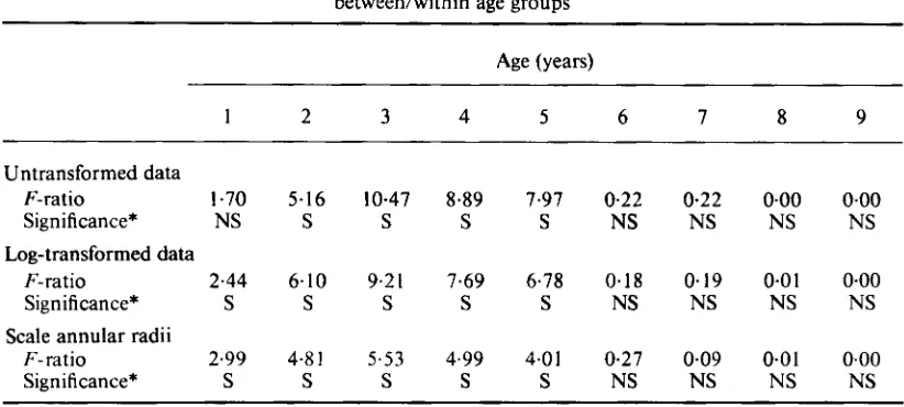
21 1

TABLE VI.

F-ratio obtained from ANOVA of back-calculated lengths and scale annular radii

betweedwithin age groups

~ ~ ~~

1

2 3 4 5 6 7 8 9

Untransformed data

F-ratio 1.70 5.16 10.47 8-89 7-97 0.22 0.22 0-00 0.00

Significance* NS S S S S NS NS NS NS

Log-transformed data

F-ratio 2.44 6.10 9.21 7.69 6.78 0.18 0.19 0.01 0.00

Significance* S S S S S NS NS NS NS

Scale annular radii

F-ratio 2.99 4.81 5.53 4.99 4.01 0.27 0.09 0.01

0.00

Significance* S S S S S NS NS NS NS

*S= Significant at

zyxwvutsrqponmlkjihgfedcbaZYXWVUTSRQPONMLKJIHGFEDCBA

P < 0.05 level; NS=not significant.

V. DISCUSSION

In the example given, linear regression analysis of the body length : scale-radius relationship of the fish population showed a significantly good fit to the data taken as a whole. Back-calculation would conventionally proceed using the parameters of this regression line.

A more detailed description of the relationship was provided by analysis of covariance which demonstrated that, although a straight line could be fitted to the data, the true trend was significantly non-linear. Following transformation of the data to logarithms a second analysis of covariance showed the transformed data to have an overall linear trend and provided the equation of that line.

A comparison of the back-calculated results obtained from parameters of the regression equations based on the untransformed and logarithmic data (expressions 2 and 17, and Tables I1 and V, respectively) is shown in Fig. 3. The two sets of results show significant differences in mean estimated length at 1 and 2

years of age, whereas the 95% confidence limits of the estimated means overlap

at

zyxwvutsrqponmlkjihgfedcbaZYXWVUTSRQPONMLKJIHGFEDCBA

3 years of age and above.

Table VI shows that S.D. between back-calculated lengths derived from fish of

different age groups occur in both the linear and logarithmic relationships. Esti- mated body lengths at 2, 3, 4 and 5 years of age show S.D. between age groups

(P<0.05) relative to within group variation in both relationships, whereas at 1

year S.D. occurs only within the log-transformed data. This could indicate the

presence of Lee’s Phenomenon (Lee, 1920) ofapparent change in growth rate with age at capture within the data if a significant trend across the range of age groups were also demonstrated (Bagenal & Tesch, 1978).

[image:11.468.33.444.84.269.2]

(12)

212

zyxwvutsrqponmlkjihgfedcbaZYXWVUTSRQPONMLKJIHGFEDCBA

J . R. BARTLETT

E T A L .

v

I I l l l l l l L

3

6

9

Age (years)

FIG. 3. Relationship between mean body length and age of fish ofa sample of 8 1 roach, Rutilus rutilus,

obtained from the parameters of regression equations fitted to the untransformed (0) and logarithmic (V) data.

This might suggest the logarithmic model to be less appropriate than the linear expression. However, S.D. also exists between age groups in the data of the first annular radius showing this to be inherent in the original data rather than an artefact of transformation.

To conclude, the use of analysis of covariance, unlike the conventional use of regression analysis, offers a detailed description of the body length : indicator relationship within a sample of data and provides an objective basis for the choice of mathematical expression to be used in back-calculation.

This paper has attempted to provide a systematic basis to the choice of back- calculation method to replace a more arbitrary approach.

The authors wish to thank Mr M. Noot for the provision of the data which is quoted

This paper is based upon work conducted under the tenure of a N.E.R.C. postgraduate

by kind permission of Dr P. B. Spillett of the Thames Water Authority.

studentship.

References

Bagenal, T. B. & Tesch, F. W. (1978). Age and growth. In Methods,for Assessment

zyxwvutsrqponmlkjihgfedcbaZYXWVUTSRQPONMLKJIHGFEDCBA

qf

(13)

BACK-CALCULATION OF GROWTH 213

Carlander, K. D. (198 1). Caution on the use of the regression method of back calculating

Dahl, K. (1909). The assessment of age and growth in fish.

Int. Revue ges. Hydrobiol.

Fraser. C. McL. (1916). Growth of the spring salmon. Trans. Pacif: Fish.

Soc.. Seattle

Graham, M. (1929). Studies of age-determination in fish. Part

zyxwvutsrqponmlkjihgfedcbaZYXWVUTSRQPONMLKJIHGFEDCBA

11. A survey of the litera-

Hile. R. (1941). Age and growth of the rock bass, Ambloplites rupestris (Rafinesque), in

Hile, R. (1970). Body-scale relation and calculation ofgrowth in fishes. Trans. A m . Fish.

Lagler, K. F. (1956). Freshwater Fishery Biology. Dubuque, Iowa: W. C. Brown. pp. 42 1.

Lea, E. (19 10). On the methods used in herring investigations. Pubfs Circonst. Cons. perm.

int. Explor. Mer 53, 7-25.

Lee, R. M. (1912). An investigation into the methods of growth determination in fishes

by means of scales. Publs Circonst Cons. perm. int. Explor. Mer 63, 3-35.

Lee, R. M. (1920). A review of the methods of age and growth determination by means

of scales. Fishery Invest., Lond., Ser. 2 4(2), 32.

Monastyrsky, G . N . (1930). 0 metodakh opredeleniya lineinogo rosta PO cheshure ryb.

(Methods of determining the growth in length of fish by their scales). Trudy Nauch.

Inst. ryb. Khoz.

zyxwvutsrqponmlkjihgfedcbaZYXWVUTSRQPONMLKJIHGFEDCBA

5 , 4.

Weatherley, A. H. ( 1 972). Growth and Ecology

of Fish Populations. London: Academic

Press. pp. 293.

Wooland, J. V.

& Jones, J. W. (1975). Studies on the grayling Thymallus thymallus (L.)

in Llyn Tegid and the upper River Dee, North Wales. 1. Age and Growth. J . Fish

Biol. 7, 749-113.

lengths from scale measurements. Fisheries 6, 2-5.

Hydrogr. 2,4-5, 758-769. 1915,29-39.

ture. Fishery Invest., Lond., Ser. 2 11(2), 50 pp.

Nebish Lake, Wisconsin. Trans. Wis. Acad. Sci. Arts. Lett. 33, 189-337.