Deflection Prediction on Machining Thin- Walled Monolithic Aerospace Component.

(1)

Delection Prediction on Machining Thin-Walled Monolithic Aerospace Component

ISSN: 2180-1053 Vol. 3 No. 1 January-June 2011 23

Deflection PreDiction on Machining

thin-WalleD Monolithic aerosPace coMPonent

r. izamshah r.a1,2, John P.t Mo1, songlin Ding1

1_{School of Aerospace, Mechanical and Manufacturing Engineering,}

RMIT University, Australia

2_{Faculty of Manufacturing Engineering,}

Universiti Teknikal Malaysia Melaka, Malaysia

Email: 1_{izamshah@utem.edu.my}

ABSTRACT

Structural titanium alloys are coming in for increased use because they are light, ductile and have good fatigue and corrosion-resistance properties As a result; more manufacturing engineers are learning that machining these alloys can be a tricky job due to their unique physical and chemical properties. The problems are worsened when machining with the low-rigidity part which makes the precision diicult to master. This paper consist of two parts, a new CAD/CAE/CAM integrated methodology for predicting the surface errors when machining a thin-wall low rigidity component and secondly, the statistical analysis to determine the correlation between a criterion variable (form errors) and a combination of a predictor (cuting parameters and component atributes). The proposed model would be an eicient means for analysing the root cause of errors induced during machining of thin-wall parts and provide an input for downstream decision making on error compensation. A set of machining tests have been done in order to validate the accuracy of the model and the results between simulation and experiment were found in a good agreement

KEYWORDS: CAD/CAE/CAM, Thin-walled work piece, Titanium alloys, Delection analysis

1.0 introDUction

The aerospace industry is the single largest market for titanium products primarily due to the exceptional strength to weight ratio, elevated temperature performance and corrosion resistance. Titanium

applications are most signiicant in jet engine and airframe components that are subject to temperatures up to 1100° F and for other critical

structural parts [1]. Usage is widespread in most commercial and military

(2)

ISSN: 2180-1053 Vol. 3 No. 1 January-June 2011 Journal of Mechanical Engineering and Technology

24

of titanium are efectively utilized. As new titanium products, alloys and manufacturing methods are employed by the aircrat industry, the

use of titanium will expand. Today the use of precision castings and machining technique are making it possible for more complex shaped

component to be made in one piece to replace ineicient assembly of

part into structures. These components have the characteristics of thin-wall monolithic part which typically being manufacture by machining the features out of one large titanium block.

Thin-wall machining of monolithic parts allows for higher quality and precise parts in less time, impact business issues including inventory

and Just-In-Time (JIT) manufacturing. Because of the poor stifness of

thin-wall part, deformation is more likely to occur in the machining of thin-wall part which resulting a dimensional form errors. In current industry practice, the resulting errors are usually compensated through one or more of the following techniques: (i) using a repetitive feeding

and inal ‘loat’ cut to bring the machined surface within tolerance; (ii) manual calibration to determine ‘tolerable’ machining conditions; and

(iii) a lengthy and expensive trial and error numerical control validation process [2]. Noticeably all of these existing techniques have a tendency

to lower productivity. With the forecast of 13,000 new aircrat will be manufacture over the next 20 years, the need for more cost efective

manufacturing method for titanium monolithic component is imminent. Therefore, the prediction of resulting surface errors when machining thin-wall monolithic component is crucial in order to increase the part accuracy and productivity.

Accuracy of machined components is one of the most critical considerations for many manufacturers especially in aerospace industry where most of the part used a thin-walled structure. Error comes from deformation of thin-walled during machining and has been largely

ignored by CAD/CAM sotware developers. The strong demand of titanium monolithic component usage has atracting many researchers in this ield especially to improve the manufacturing eiciency. Current

problems in thin-walled machining are that most of these works were conceptual and considered only parts with a simple geometry such as rectangular plate. This is due to the nature of the limitation in design

lexibility to create complex part in FEA sotware. Alternatively, the complex geometry oten been generated from CAD sotware and transferred to the FEA sotware with a neutral database form such as

IGES, DXF, VDA, STEP and STL. However, owing to the exchanging

data of diferent platform can cause some problems such as loss of data

organization, translation inaccuracies, change in number of entities

(3)

ISSN: 2180-1053 Vol. 3 No. 1 January-June 2011 25 same working environment is essential to minimize the possible error when exchanging data and to maintain associativity with the master design. Associativity includes time for remeshing the product model

for analysis, the iterative loop of computing forces and delections. This is not practical when the technique is used on shoploor.

This paper proposes a new model for predicting the part delection

when machining thin-walled work piece. The paper consist of two

parts, irst, an integrated CAD/CAE/CAM methodology for predicting

the surface errors when machining a thin-wall component and secondly, the statistical analysis to determine the correlation between

a criterion variable (part delection) and a combination of a predictor (cuting parameters and component atributes). The system integration

consists of machining load computational model from the machining parameter, feature based geometry model, material removal model,

delection analysis model and NC machining veriication model. The

proposed CAD/CAE/CAM methodology is implemented with CATIA V5 platform using the Mechanical Design workbench, Generative Structural Analysis workbench, Advanced Meshing workbench and Machining workbench.

2.0 literatUre revieW

There were few reported work been done in predicting the deformation of thin-wall part. Budak and Altintas [3] used the beam theory to analyse the form errors when milling using slender helical endmill for peripheral milling of a cantilever plate structure. The slender helical endmill is divided into a set of equal element to calculate the form

errors acting by the cuting forces on both tool and the workpiece.

Kline et.al. [4] used a thin-wall rectangular plate element model clamped on three edges. He used an equivalent concentrated force to

calculate the delection of the tool and the work piece. The form errors are obtained by summing the tool and the work piece delection. The efects of workpiece and cuter dynamic delections on the chip load

are proposed by Elbastawi and Sagherian [4]. Included in their model

is the tracking of the changing of dynamics stifness of workpiece geometry. In addition, the efects of cuter delection for estimating the

instantaneous uncut chip thickness were proposed by Sutherland and Devor [5]. Later, Tsai and Liao [6] developed an iteration schemes to

predict the cuting forces and form error on thin-wall rectangle plate. The cuting force distribution and the cuting system delections are solved iteratively by modiied Newton-Raphson method. Ratchev

(4)

26

for machining low-rigidity components. Later in his work, Ratchev

et.al. [8] modelled the material removal process using voxel-based

representations by cuting through the voxels at the tool/part contact

surface and replacing them with equivalent set of mesh. He used

Aluminium Alloys 6082 for the experimental analysis and veriication. Rai and Xirouchakis [9] consider the efects of ixturing, operation

sequence and tool path in transient thermo-mechanical coupled milling simulation of thin-walled components. Recently, Izamshah et.al. [10] adopted the Lagrangian method in his machining simulation, in which each individual node of the mesh follows the corresponding material

particle during motion. The workpiece is modelled as a plastic object so

that the material can be deform and cut by the endmill teeth.

Despite of several signiicant works on modelling thin-wall machining that has been developed, there still a requirement for more eicient

approach on modelling the thin-wall machining especially for minimizing the analysis time from initial part creation to analysis result. The advantages of the proposed model over previous work are the integration between CAD/CAE/CAM, fast design-analysis

loop and the lexibility to create complex inite element models while

maintaining associativity with the master design, thereby avoiding time-consuming and error-prone transfer of geometry.

3.0 MoDelling anD siMUlation systeM architectUre

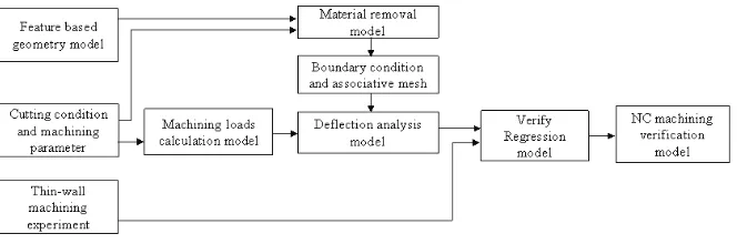
The proposed modelling and simulation system architecture for machining thin-wall components is shown in Figure 1. The system consist of several model, namely, machining load computational model derived from the machining parameter, feature based geometry

model, material removal model, delection analysis model and NC machining veriication model. The methodology is performed within

the CAD environment and the analysis model is fully associative

with the CAD geometry and speciication. MATLAB sotware was

used in machining load computational model while others models

were implemented using CatiaV5 sotware using Mechanical Design

workbench, Advanced Meshing workbench and Generative Structural Analysis workbench. The simulation is perform by automate the task

for modelling solids object, material removal and structural analysis

with CatiaV5 through the use of macros, with Windows as the operating system and Visual Basic as the programming language In addition multiple regression technique is used to perform the statistical analysis

(5)

ISSN: 2180-1053 Vol. 3 No. 1 January-June 2011 27 and a combination of predictor variables. Finally, both models were validating with a set of machining tests. The methodology consists of

several procedures with diferent functions as follows:

Machining load computational model

In the machining load computational model, the machining parameters

and tool geometry, namely, cuting speed (rpm), radial depth of cut, axial depth of cut, feed rate (mmpt), tool diameter, helix angle (β) and speciic cuting forces (Kt and Kr) are used as an input to calculate the

machining loads. The procedure to calculate the machining load is described later in Section 3.1. The calculated machining loads is stored and saved in a native ASCII ile format and will be used as an input in

the delection analysis model. β

FIGURE 1: Modelling and simulation system architecture. FIGURE 1: Modelling and simulation system architecture.

feature based geometry model

The component feature atributes such as the initial workpiece

dimensions and material properties are created in the Catia Mechanical Design workbench. The part is created by automating the task for

modelling solids object with Catia V5 through the use of macros, with

Windows as the operating system and Visual Basic as the programming language. By using a simple form the dimension are enter which

deine the geometry of the part (length, thickness and height). This

application automatically and immediately creates the part compare with the manual process that would require construction of lines and generation of solid model. The created component is saved in CATPart

ile format and work as a master design. Any changes and update of

material removal need to be done in this master design.

Material removal model

(6)

28

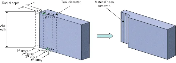
material will be remove using extrude (cut) and array function in the Catia Mechanical Design workbench as shown in Figure. 2. For

the irst step, the cuter is set at the entry of the workpiece and the material which is coincidence with the cuter shape are remove and

saved as a new CATPart ile. Once the cuter feed position is deined, the component feature will be input to Catia Advanced Meshing Tool workbench for generation of associative mesh for the solid component. At this stage, global parameters such as the shape and the size of the

elements needs to be specify to perform the inite element analysis. Delection analysis model

Catia Generative Structural Analysis workbench are use to perform

a static analysis for part delection prediction. At this phase analysis

information such as nodes, elements, material properties, boundary conditions and the calculated machining load will be input to calculate

the delection. The procedure to calculate the part delection is described

later in Section 3.2. The FEA results which contain the elements and nodes values is stored and saved in a native ASCII ile format and saved

in CATAnalysis ile and stored in a knowledge-based template. The cuter

feed position is then move to the next position and the material on the new feed step will be removed to perform the subsequent analysis.

Finally, ater repeating this procedure at diferent location along the

feed direction, the complete surface form errors of the component are obtained and are used in Catia Machining workbench for tool path

compensation and NC veriication.

NC machining veriication model

Once the complete surface form errors of the thin-wall are obtain, the

tool paths can be corrected to compensate for machining error. The compensation is done by mirroring the surface error in the opposite

direction of the wall delection along the feed direction. On the other

(7)

ISSN: 2180-1053 Vol. 3 No. 1 January-June 2011 29 FIGURE 2: CAD based material removal model for machining.

3.1 Machining load model for helical endmill

As shown in Figure 3, the machining loads acting on a helical lute endmill are equally discretized into a inite number of elements along the tool axis. The total cuting loads (F_x, F_y and F_z) acting on the tool at a particular instant are obtain by summing the force components acting on each individual discretized element [16, 17, 18].

FIGURE 3: Cutting force model for helical endmill.

( )φ = ( )φ +

φ

( )φ = φ( ) ( )

φ

χ

( )( )γ χ=

FIGURE 3: Cuting force model for helical endmill.

( )

z K h

( )

z K z dFtjφ, =[ tc jφ, + te]d ,

( )

z K h

( )

z K z dFrjφ, =[ rc jφ, + re]d ,

dFaj

( )

φ,z =[Kachj

( )

φ,z +Kae]dz

are differential forces corresponding to discretiz al and axial directions. The coefficients K , K , K and

φ

( )

φ = φ

( )

φ

χ

( )( )

γ χ=

( )

φ =

( )

φ +

( )

φ =

( )

φ +

( )

φ =

( )

φ + (1)

ment thickness in are the spec

φ

( )

φ = φ

( )

φ

χ

( )( )

γ χ=

where dF

tj, dFrj and dFaj are diferential forces corresponding to

discretized element thickness in the tangential, radial and axial

directions. The coeicients K

tc, Krc, Kac and Kte, Kre, Kae are the speciic

cuting force coeicients and speciic edge cuting force coeicients

to each tangential, radial and axial direction, determined from the experimental analysis.

( )

φ =

( )

φ +

( )

φ =

( )

φ +

( )

φ =

( )

φ +

ng force coefficien tal analysis. φ is th

cut chip thickness for the fl

( )

φ = φ

( )

φ

χ

( )( )

γ χ=

is the tool’s immersion angle start from

positive y-axis and h_j is the instantaneous uncut chip thickness for the

(8)

30

( )

φ =

( )

φ +

( )

φ =

( )

φ +

( )

φ =

( )

φ +

φ

hj

( )

φ,z = ftsinφj

( )

z tooth and φj

( )

z is the entry and exit angl

χ

( )( )

γ χ=

( )

φ =

( )

φ +

( )

φ =

( )

φ +

( )

φ =

( )

φ + φ

( )

φ = φ

( )

(2)

( )

φ at certain position

χ

( )( )

γ χ=

where f_t is the feed per tooth and

( )

φ =

( )

φ +

( )

φ =

( )

φ +

( )

φ =

( )

φ +

φ

( )

φ = φ

( )

per tooth and φj

( )

z is t

rection. Since this study using a h

the same instant and χ

( )( )

γ χ=

is the entry and exit angle for

lute j at certain position in the axial direction. Since this study using a

helical cuter the full length of the cuting edge does not enter (or exit)

the cut at the same instant and the angular delay between disretize elements

( )

φ =

( )

φ +

( )

φ =

( )

φ +

( )

φ =

( )

φ + φ

( )

φ = φ

( )

φ

tting edge does n elements χcan be

( )( )

γ χ=

can be approximated as follows: ( )φ = ( )φ + ( )φ = ( )φ + ( )φ = ( )φ + φ ( )φ = φ( ) ( ) φ χ

oximated as follows:

FIGURE 4: Discretized unrolled helical endmill geometry.

( )( )γ χ =

FIGURE 4: Discretized unrolled helical endmill geometry.

( )

φ =

( )

φ +

( )

φ =

( )

φ +

( )

φ =

( )

φ + φ

( )

φ = φ

( )

φ χ

( )( )

rad r db γ

χ= tan

( )

φ =

( )

φ +

( )

φ =

( )

φ +

( )

φ =

( )

φ + φ

( )

φ = φ

( )

φ χ

( )( )

γ

χ= (3)

where r is the tool diameter, diameter, γis h

φfor χyields:

( )

γ φ = ( )φ =− _γ[− φ+ φ( )− φ( )] ( )( )φφ ( )φ =− _γ[φ( )− φ( )+ φ( )] ( )( )φφ ( )φ =− _γ [ φ( )] ( )( )φφ

( )

φ

( )

φ δ δ δ

is helix angle and db is the element thickness. Rearranging Eqs. (3) and substituting

γ bstituting dφfor χ

( )

φ

( )

φ δ δ δ for γ ting φfor χyie

( )

φ

( )

φ δ δ δ yields: γ φ χ ( )γ φ tan .d r db= ( )φ =− _γ[− φ+ φ( )− φ( )] ( )( )φφ ( )φ =− _γ[φ( )− φ( )+ φ( )] ( )( )φφ ( )φ =− _γ [ φ( )] ( )( )φφ ( )φ ( )φ δ δ δ γ φ χ ( )γ φ = (4) ( )φ =− _γ[− φ+ φ( )− φ( )] ( )( )φφ ( )φ =− _γ[φ( )− φ( )+ φ( )] ( )( )φφ ( )φ =− _γ [ φ( )] ( )( )φφ ( )φ ( )φ δ δ δ

By substituting and integrating the diferential cuting forces from Eqs. (1) to (4) within the lower and upper boundaries of the lute which is in

cut. The tangential, radial and axial forces can be transformed in x, y, z Cartesian directions and becomes:

γ φ χ ( )γ φ = ( )φ _γ[ φ φ( ) φ( )] ( )( )φφ Zju Zjl j j r j t t

xj Kfr K z z

F cos2 (2 sin2 )

tan

4 − + −

− = ( )φ _γ[φ( ) φ( ) φ( )] ( )( )φφ Zju Zjl j r j j t t

yj Kfr z z K z

F 2 sin2 cos2

tan

4 − +

− = ( ) [ ( )] _{( )}( )φ φ φ γ φ Zju Zjl j t t a

zj KKfr z

F cos tan − = ( )φ ( )φ δ δ δ γ φ χ ( )γ φ = ( )φ =− _γ[− φ+ φ( )− φ( )] ( )( )φφ ( )φ =− _γ[φ( )− φ( )+ φ( )] ( )( )φφ

( )φ =− _γ [ φ( )] ( )( )φφ (5)

( )φ ( )φ

δ δ δ

where Zjl(

( )

φ =

( )

φ +

( )

φ =

( )

φ +

( )

φ =

( )

φ +

ng force coefficie tal analysis. φ is th

cut chip thicknes

( )

φ = φ

( )

φ χ

( )( )

γ χ=

) and Zju(

( )

φ =

( )

φ +

( )

φ =

( )

φ +

( )

φ =

( )

φ +

ng force coefficien tal analysis. φ is th

cut chip thicknes

( )

φ = φ

( )

φ χ

( )( )

γ χ=

) are the lower and upper axial engagement limits

of the in cut immersion of the lute j. From Eqs. (5) the instantaneous

(9)

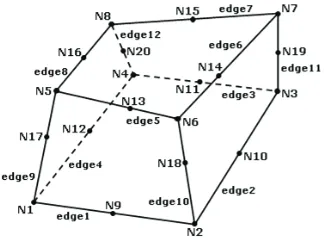
3.2 finite element modelling of thin-wall workpiece

The structural of the thin-wall workpiece is modelled with the three-dimensional twenty-node parabolic hexahedron solid element as shown in Figure 5. Parabolic hexahedron solid element is preferred since the thickness of the wall is very thin and the change in structural properties of the wall due to material removed is very important for

accurate prediction of the wall delections [16, 17]. For the

three-dimensional element, each node has three degrees of freedom, i.e,

three displacements (δ_x, δ_y and δ_z) and the displacements within

each element are interpolated by the nodal values [18].

γ

φ χ

( )

γ φ =

( )φ =− _γ[− φ+ φ( )− φ( )] ( )( )φφ

( )φ =− _γ[φ( )− φ( )+ φ( )] ( )( )φφ

( )φ =− _γ [ φ( )] ( )( )φφ

( )

φ

( )

φ

δ δ δ

FIGURE 5: Parabolic hexahedron solid element. FIGURE 5: Parabolic hexahedron solid element.

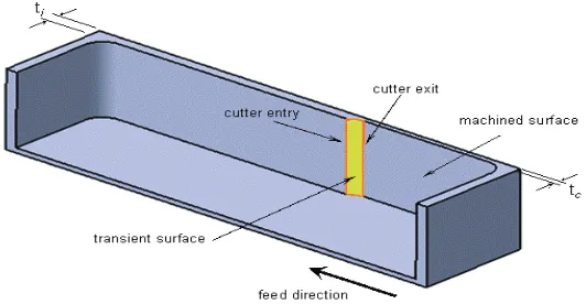
Figure 6 shows the thin-wall component model for delection

calculations. The initial wall thickness t_i is reduced to t_c at the

transient zone where the cuter lutes enter and exit the material

in the milling process. The displacements of the whole structure

component are obtained by assembling and solving the inite

element equations for each element together as follows:

[ ]

Kwpnwp x nwp

{ }

δ nwp x 1=

{ }

F nwp x 1

[ ]

{ }

δ

{ }

β β β β β β β

[ ]

{ }

δ =

{ }

(6)

[ ]

{ }

δ

{ }

where

[ ]

{ }

δ

=

{ }

where

[ ]

K

wp nwp x nwp

is the

{ }

δ

workpiece and

{ }

F

β

is the stifness matrix of the workpiece,

[ ]

{ }

δ

=

{ }

[ ]

workpiece,

{ }

δ

nwp x 1

is the

{ }

ting force acting on

β

is the nodal displacement of the workpiece and

[ ]

{ }

δ

=

{ }

[ ]

is the stiffness

{ }

δ

iece and

{ }

F nwp x 1 is th

rkpiece calculated in Secti

is the vector

of the cuting force acting on the transient surface of the workpiece

calculated in Section 3.1. The nodal displacement for the structural

component can be solved by deining the displacement boundary

(10)

32

[ ]

{ }

δ =

{ }

[ ]

{ }

δ

{ }

Figure 6: Modelling the thin-wall component.

3.3 statistical analysis

Multiple regression technique is used to perform the statistical analysis

to determine the correlation between a criterion variable; part delection

and a combination of a predictor variables namely speed, feed rate, radial depth of cut, wall thickness, wall height and wall length. It can

be used to analyse data from any of the major quantitative research

designs such as causal-comparative, correctional and experimental. This method is also able to handle interval, ordinal, or categorical data

and provide estimates both of the magnitude and statistical signiicance

of the relationship between variables [15]. The multiple regression models can be expressed as:

[ ]

{ }δ ={ }

[ ]

{ }δ

{ }

yD1, D2, D3, D4 ,D5 = β0 + βSS + βFF + βRDOCRDOC + βWPTWPT + βWPHWPH + βWPLWPL (7)

where

y = displacement (µm) at D1_,D2_,D3_,D4_andD5

S_{= Speed (rpm)}

F_{= Feed rate (mmpt)}

RDOC = Radial depth of cut (mm) WPT = Workpiece thickness (mm) WPH = Workpiece height (mm) WPL = Workpiece length (mm)

The general null hypotheses was described as the efects of speed, feed

rate, radial depth of cut, workpiece thickness, workpiece height and

(11)

ISSN: 2180-1053 Vol. 3 No. 1 January-June 2011 33 Ho = βS=βF=βRDOC=βWPT=βWPH=βWPL= 0

Ha = at least one of the βdoes not equal to zero

The regression analysis is veriied by using the residual plot graph,

which shows the residuals on the vertical axis and the independent variable on the horizontal axis. If the points in a residual plot are randomly dispersed around the horizontal axis, a linear regression

model is appropriate for the data; otherwise, a non-linear model is

more appropriate.

4.0 nUMerical anD exPeriMental Work

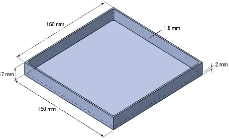
The proposed CAD/CAE/CAM integrated methodology for minimizing the surface errors when machining a thin-wall low rigidity component was experimentally tested by comparing the simulation results with the results of experiment for an identical set of test components. The geometry of the component used in the simulation and experiment is shown in Figure 7. Twenty-node parabolic hexahedron solid element

is used to discretized the component for FE model. Only the botom

face of the component is clamped and the other four sides are free.

The authors have tested three uniform inite element meshes for the

component wall, 100x1x10, 200x2x20 and 300x4x40 (number of elements in X-direction) x (number of elements in Y-direction) x (number of elements in Z-direction), the numerical results for the 200x2x20 and 300x4x40 meshes were being very close. Hence, 200x2x20 is adopted as

the inite element mesh to save the computational time. The component

was predicted and measured at 30 equally space at one side of the wall along the feed direction. The radial depth of cut is 0.3 mm and the axial depth of cut is 15 mm.

β β β β β β

β

FIGURE 7: Work piece dimension for simulation and experimental.

(12)

34

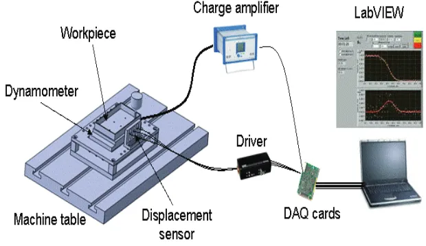
The experimental set-up is shown in Figure 8. All experimental tests were performed on a HAAS VF1 vertical machining center. Three component Kistler dynamometer (type 9257B) and Kistler charge

ampliier (type 5070A) are used to measure the cuting loads, while

National Instrument DAQ card is used to acquire the signal. The wall

delection is measured using three Lion Precision ECL 130 inductive displacement sensors. The sensors are mounted at three diferent equal

locations (37.5, 75 and 112.5 mm) at the back of the workpiece. Both the signals from the dynamometer and displacement sensors are then been analyse using LabVIEW 8.5.1.

FIGURE 8: Experimental set-up. FIGURE 8: Experimental set-up

The workpiece material used in the simulation and experimental is annealed alpha-beta titanium alloy, Ti-6Al-4V. The chemical composition and mechanical properties of the material is shown in Table 1 and 2,

respectively. Table 3 shows the speciication of carbide lat end mills

used in the experiment. To perform the multiple regression analysis, a set of 27 runs on titanium alloys were generated from Section 3.2.

The cuting parameters data were obtained from the industrial partner Production Parts Pty. Ltd. Australia, for inishing cycle on machining

titanium alloys material. Table 4 shows the 6-Factors 3-Level design of experiment for the multiple regression analysis. The criterion

variable are calculated at ive diferent location along the workpiece

(13)

ISSN: 2180-1053 Vol. 3 No. 1 January-June 2011 35 TABLE 1: Chemical compositions of Ti-6Al-4V alloy (wt. %)

Chemistry N C H O Fe Al V Ti Other elements % w/w, min. - - - - - 5.50 3.50 - -

% w/w, max. 0.05 0.10 0.0125 0.20 0.30 6.75 4.50 Balance 0.40

TABLE 2: Mechanical properties of Ti-6Al-4V alloy at room temperature.

Density Young’s modulus Poisson ratio Yield strength Hardness Elongation [kg/m3_] _[GPa] _{[MPa] [HB]} _[%] 4430 113.8 0.34 880 334 14

TABLE 3: Cuting tool speciication.TABLE 3: Cutting tool specification.

D d Ap H L Flute Ha° Rd° Shank Ch 6.00 6.00 14.00 20.00 57.00 4 38.0 5.0 C 0.25X45

TABLE 4: Design of experiment for the multiple regression analysis.TABLE 4: Design of experiment for the multiple regression analysis. Level 1 Level 2 Level 3

Speed (rpm) 4244 4509 4774

Feed rate (mmpt) 0.02 0.05 0.08 Radial depth of cut (mm) 0.1 0.2 0.3

WP Thickness (mm) 1.5 2 2.5

WP Height (mm) 5 10 15

WP Length (mm) 60 90 120

5.0 cUtting loaDs valiDation

MATLAB 7.7 was used for the machining loads computational as

described in Section 3.1. To validate the cuting loads model, the predicted forces are compared with measured forces for inishing cycle.

As in Section 3.1, the milling forces can be transformed in x, y and z. However, for the case of thin-wall machining, the force acting in the

opposite direction of the wall is speciically considered as it has major impact on the wall delection, which in this case is F_y. The wall thickness is to be reduced from 1.8 mm to 1.5 mm with 3500 rpm spindle speed and a feed rate of 0.05 mm feed per tooth which is constant along the

feed direction. Others machining parameters are wall height is 17 mm,

(14)

36

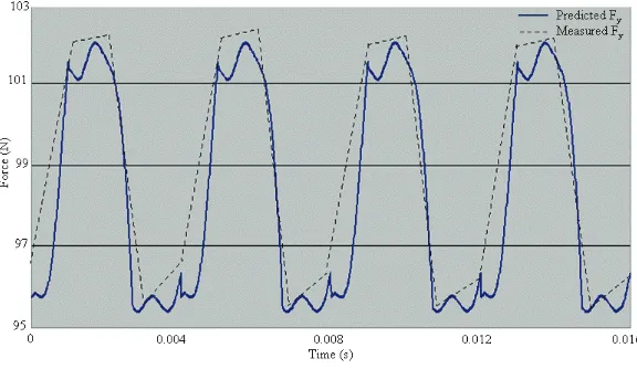
piece material is titanium alloys. Figure 9 shows the instantaneous predicted and measured force F_y for one cuter revolution. As it can be clearly observed, both the values between predicted and measured force are in a good agreement. The calculated machining loads will be

use as an input for the FEA to calculate the delection of the work piece

during machining.

FIGURE 9: Calculated cutting force for one cutter revolution.

FIGURE 9: Calculated cuting force for one cuter revolution.

5.1 Part delection validation

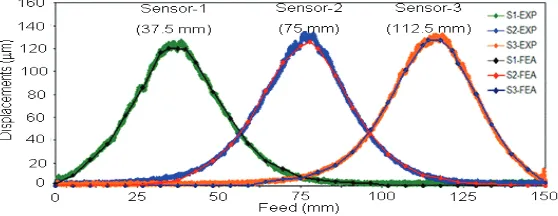
Figure 10 shows the displacement values for three sensors between

simulation and experiment. The cuter feed step is set at 30 equally

space location at one side of the wall along the feed direction. The material from the previous feed step need to be removed once the

cuter move to the next feed step. Table 5 shows the errors calculation

between predicted and measured value. It can be seen that both the displacement obtained by simulation closely match the displacement that are obtained by experiment. The agreement value between predicted and measured is between 80.3% and 99.9%. Figure 11 shows the simulation result of the displacement magnitudes at the middle

location of cuter feed step. From the cut plane analysis of the wall, it shows that the form errors are smallest at the botom of the part.

The form errors magnitudes increase towards the middle of the part

and decrease towards the end of the part, where the wall lexibility decreases. Due to the decreasing stifness of the wall as a result of

material removal, there is an increasing value of form errors between two regions (start and end) in the feed direction. To a large extent, the

(15)

the resulting proile error, the cuter location needs to be modiied from

the initial position to the compensated position by a distance of the

resulting displacement value at certain cuter feed position.

FIGURE 10_{FIGURE 10: Comparison between simulation and experiment of}: Comparison between simulation and experiment of displacement along the

displacement along the workpiece length.

TABLE 5: Error calculations between prediction and measured value.

Feed (mm)

S1 S2 S3

FEA EXP Agreement FEA EXP Agreement FEA EXP Agreement

0 1.839 1.701 91.9 0.001 0.001 87.1 1.82E-04 1.98E-04 91.8

5 9.135 9.880 92.5 0.006 0.007 88.5 3.96E-04 3.37E-04 82.5

10 22.841 23.164 98.6 0.044 0.050 88.1 1.94E-03 1.67E-03 83.8

15 36.505 37.627 97.0 0.175 0.208 84.1 3.56E-03 3.96E-03 89.9

20 61.598 61.419 99.7 0.427 0.362 82.0 6.29E-03 6.77E-03 92.9

25 86.071 85.222 99.0 1.016 1.201 84.6 1.01E-02 1.12E-02 89.9

30 116.508 116.029 99.6 2.625 3.035 86.5 1.45E-02 1.51E-02 96.3

35 119.971 121.016 99.1 5.014 5.676 88.3 1.78E-02 1.72E-02 96.4

40 107.952 107.357 99.4 12.702 13.234 96.0 1.97E-02 1.72E-02 85.5

45 82.116 81.632 99.4 21.805 22.047 98.9 2.20E-02 2.22E-02 98.8

50 58.810 58.456 99.4 35.995 36.286 99.2 0.118 0.147 80.3

55 36.920 37.285 99.0 55.582 55.121 99.2 0.259 0.312 83.0

60 21.694 21.642 99.8 82.868 82.075 99.0 3.415 3.594 95.0

65 14.727 14.155 96.0 108.051 107.861 99.8 5.909 6.051 97.7

70 7.608 7.816 97.3 120.119 123.653 97.1 6.603 6.731 98.1

75 5.280 5.156 97.6 120.017 121.749 98.6 11.757 11.940 98.5

80 3.654 3.724 98.1 96.585 95.843 99.2 17.924 18.047 99.3

85 2.750 2.798 98.3 68.106 67.111 98.5 29.754 29.788 99.9

90 2.291 2.153 93.6 45.251 44.592 98.5 48.877 48.023 98.2

95 3.35E-02 3.49E-02 95.9 27.389 27.602 99.2 72.829 72.790 99.9

100 2.68E-03 2.82E-03 95.1 17.132 17.359 98.7 101.257 100.619 99.4

105 1.25E-03 1.41E-03 88.7 9.381 9.656 97.2 119.910 122.700 97.7

110 1.22E-03 1.24E-03 98.4 6.644 6.908 96.2 119.689 122.300 97.9

115 9.34E-04 9.53E-04 98.0 3.392 3.487 97.3 107.051 107.523 99.6

120 6.18E-04 6.86E-04 90.1 2.043 2.002 98.0 80.345 80.461 99.9

125 3.72E-04 3.96E-04 93.9 1.493 1.583 94.3 53.641 53.071 98.9

130 1.97E-04 2.02E-04 97.5 0.906 1.109 81.7 27.968 28.422 98.4

135 1.82E-04 1.90E-04 95.8 0.015 0.013 90.3 14.252 14.131 99.1

140 1.78E-04 1.81E-04 98.3 0.003 0.003 85.4 2.445 2.455 99.6

(16)

38

(a) (b)

(c)

FIGURE 11: (a) Machining simulation for displacement analysis of the test part at the middle location of cuter feed. (b) Cut plane analysis of

the part. (c) Back view of the part.

5.2 Multiple regression analysis

A set of 27 runs were generated from Section 3.2 to perform the regression analysis. Table 6 shows the training data set for the parameters and the

displacements at ive diferent locations along the cuter feed position. Assumptions of normality and independence of residuals were irst

checked using a normal probability and residual plot. The normal probability plot of the residuals for displacement at D1, D2, D3, D4 and D5 were shown in Figure 12. In this plot, the actual data are ranked and sorted, and an expected normal value is computed and compared with an actual normal value for each case. As shown in Fig. 12, the data are spread roughly along the straight line which indicates that the normal

distribution of residuals was satisied.

(17)

ISSN: 2180-1053 Vol. 3 No. 1 January-June 2011 39 TABLE 6: Training data set for regression analysis.

SPEED (rpm)

FEED (mmpt)

RDOC (mm)

WP [t] (mm)

WP [h] (mm)

WP [l] (mm)

D1 (µm)

D2 (µm)

D3 (µm)

D4 (µm)

D5 (µm)

4244 0.02 0.1 1.5 5 60 0.0835 0.6730 0.6770 0.6740 0.0783

4244 0.02 0.1 1.5 10 90 0.1060 2.6900 2.7300 2.6900 0.0935

4244 0.02 0.1 1.5 15 120 0.1230 6.5200 6.7300 6.5900 0.1060

4244 0.05 0.2 2 5 60 0.1240 0.7620 0.7670 0.7560 0.1290

4244 0.05 0.2 2 10 90 0.1540 2.7900 2.8200 2.7800 0.1360

4244 0.05 0.2 2 15 120 0.1750 6.6000 6.7500 6.6000 0.1480

4244 0.08 0.3 2.5 5 60 0.1470 0.6780 0.6850 0.6780 0.1474

4244 0.08 0.3 2.5 10 90 0.1830 2.3000 2.3200 2.2900 0.1540

4244 0.08 0.3 2.5 15 120 0.2040 5.2600 5.3800 5.2700 0.1640

4509 0.02 0.2 2.5 5 90 0.0596 0.3170 0.3170 0.3180 0.0598

4509 0.02 0.2 2.5 10 120 0.0712 1.0200 1.0200 1.0200 0.0642

4509 0.02 0.2 2.5 15 60 0.0784 1.1200 2.2600 1.1100 0.0678

4509 0.05 0.3 1.5 5 90 0.2500 1.6500 1.6400 1.6600 0.1900

4509 0.05 0.3 1.5 10 120 0.2880 6.7400 6.7700 6.7400 0.2300

4509 0.05 0.3 1.5 15 60 0.2840 9.4200 10.014 9.4320 0.2560

4509 0.08 0.1 2 5 90 0.1210 0.7800 0.7610 0.7810 0.1190

4509 0.08 0.1 2 10 120 0.1470 2.7600 2.7700 2.7700 0.1280

4509 0.08 0.1 2 15 60 0.1660 4.9200 6.3100 4.9200 0.1380

4774 0.02 0.3 2 5 120 0.0965 0.5550 0.5510 0.5540 0.0881

4774 0.02 0.3 2 10 60 0.1250 1.8300 2.0500 1.5000 0.0968

4774 0.02 0.3 2 15 90 0.1450 4.5400 4.9400 4.5500 0.1050

4774 0.05 0.1 2.5 5 120 0.0754 0.3860 0.3860 0.3860 0.0761

4774 0.05 0.1 2.5 10 60 0.0869 1.1100 1.2300 1.1100 0.0784

4774 0.05 0.1 2.5 15 90 0.0959 2.4200 2.8500 2.6400 0.0840

4774 0.08 0.2 1.5 5 120 0.2230 1.7640 1.7700 1.7600 0.2180

4774 0.08 0.2 1.5 10 60 0.2900 5.5000 7.2000 6.3000 0.2560

4774 0.08 0.2 1.5 15 90 0.3290 9.6800 11.015 9.7600 0.2820

Figure 13 shows plotting of the residuals in time order of data collection. The purpose of this graph

Figure 13 shows ploting of the residuals in time order of data

collection. The purpose of this graph is to check the independence assumption on the residuals. It is desired that the residual plot should

contain no obvious paterns. From the graph it shows a tendency to

(18)

40

α

Figure 13: Residuals in time order for D1, D2, D3, D4 and D5.

Based on the validity of the assumptions, ANOVA was used for the regression analysis. From the ANOVA analysis, the R square obtained

from the regression analysis for displacement at D1, D2, D3, D4 and D5 were 92.3%, 86.2%, 87.6%, 85.9% and 90.7% respectively, which

indicated high correlation coeicient between the dependent variable

and the predicted value. All these evidences showed a strong linear relationship between the predictor variables (S_,F_,RDOC_,WPT_,WPH

and WPL) and the predicted variables.

The results of analysis of variance (ANOVA) of the models also

supported strong linear relationship in the models (Table 7). The calculated F values of the regression were 39.80, 20.80, 23.52, 20.34 and

32.50, respectively. These high values indicated a great signiicance (α = 0.000) for the models in rejecting the null hypothesis (H_o) that every

coeicient of the predictor variables in the model was zero. Instead, the alternative hypothesis, at least one of these coeicients did not

equal to zero, was accepted. Therefore, the linear relationship between

predicted variables and predictor variables signiicantly existed. The coeicients of all predictor variables and constants of the models are listed in Table 8. According to these coeicients, the multiple regression

models for D1, D2, D3, D4 and D5 can be writen as, respectively: D1 = 0.0005 + 0.000035S + 1.707F + 0.39878RDOC - 0.10834WPT + 0.004670WPH + 0.0000339WPL

(19)

ISSN: 2180-1053 Vol. 3 No. 1 January-June 2011 41 D4 = 1.552 + 0.000049S + 28.746F + 5.618RDOC - 3.4204WPT + 0.48117WPH + 0.009648WPL D4 = 0.0362 + 0.00002688S + 1.5672F + 0.29444RDOC - 0.09039WPT + 0.002717WPH - 0.0000469WPL

TABLE 7: Analysis of variance (ANOVA).TABLE 7: Analysis of variance (ANOVA).

Model Source Sum of Squares DF Mean square F Sig.

D1 Regression 0.140040 6 0.023340 39.80 0.000 Residual 0.011730 20 0.000586

Total 0.151770 26

R-Square 92.3

D2 Regression 172.014 6 28.669 20.80 0.000 Residual 27.571 20 1.379 Total 199.585 26

R-Square 86.2

R-Square 87.6

R-Square 85.9

D5 Regression 0.096431 6 0.016072 32.50 0.000 Residual 0.009890 20 0.000495

Total 0.106321 26 R-Square 90.7

TABLE 8: The model coeicients.TABLE 8: The model coefficients.

D1 D2 D3 D4 D5

Constant 0.0005 2.052 -0.633 1.552 0.03621

S 0.00003505 -0.000102 0.000657 0.000049 0.00002688

F 1.7070 26.624 31.672 28.746 1.5672

RDOC 0.39878 5.952 5.503 5.618 0.29444

WPT -0.10834 -3.3362 -3.5850 -3.4204 -0.09039

WPH 0.004670 0.47683 0.54291 0.48117 0.002717

WPL 0.0000339 0.010356 0.001730 0.009648 -0.0000469

6.0 conclUsions

(20)

42

the surface errors when machining a thin-wall low rigidity component and the statistical analysis to determine the correlation between a criterion variable (form errors) and a combination of a predictor

(cuting parameters and component atributes) were developed. A set

of machining tests have been done in order to validate the accuracy of the model. A good agreement between simulation and experimental

results show the validity of the proposed model in handling real-ield

problems. In addition, results from the statistical analysis showed a strong linear relationship between the predictor variables (S, F, RDOC,

WPT, WPH and WPL) and the predicted variables (surface errors).

Prediction of the surface errors due to the lexibility of the workpiece

can be easily predicted with the proposed CAD/CAE/CAM integrated

methodology. On the other hands, the advantages of the proposed model

are for minimizing the analysis time i.e. integration between CAD/CAE/ CAM, fast design-analysis loop, multidiscipline collaboration and the

lexibility to create complex inite element models while maintaining

associativity with the master design, thereby avoiding time-consuming and error-prone transfer of geometry. The CAD/CAE/CAM integrated

methodology would be an eicient means for analysing the root cause

of errors induced during machining of thin-wall parts and provide an input for downstream decision making on error compensation. To a large extent, through the CAD/CAE/CAM model, manufacturers can further enhance their productivity by eliminating the need of expensive

preliminary cuting trials oten require for validating the designed

machining process plan.

acknoWleDgeMents

This work supported by Australian Government, Department of Innovation Industry, Science and Research. The authors would like to thanks Production Parts Pty Ltd Australia, for providing the experiment material and technical supports.

references

[1] Songlin D, R. Izamshah R.A, John P.T Mo, Quansheng L., Online tool life prediction in the machining of titanium alloys, J. of Key Engineering Materials Vol. 458 (2011) 355-361.

[2] M.A Elbestawi, R.Sagherian, Dynamics modelling for the prediction of surface errors in the milling of thin-walled sections, J. of Materials Processing Technology 25 (1991) 215-228.

(21)

[4] J.W Sutherland, R.E DeVor, An improved method for cuting force and surface error prediction in lexile end milling system, ASME J. Eng. Ind. 108 (1986) 269-279.

[5] J.W Sutherland, R.E DeVor, An improved method for cuting force and surface error prediction in lexile end milling system, ASME J. Eng. Ind. 108 (1986) 269-279.

[6] J.S Tsai, C.L. Liao, Finite element modelling of static surface errors in the peripheral milling of thin-walled workpiece, J. of Materials Processing Technology 94 (1999) 235-246.

[7] S. Ratchev, W.Huang, S.Liu, A.A Becker, Modelling and simulation environment for machining of low-rigidity components, J. of Materials Processing Technology 153-154 (2004) 67-73.

[8] S. Ratchev, W.Huang, S.Liu, A.A Becker, Milling error prediction and compensation in machining of low-rigidity parts, Int. J. of Mach. Tools Manuf. 44 (2004) 1629-1641.

[9] J.K Rai, P.Xirouchakis, Finite element method based machining simulation environment for analyzing part errors induced during milling of thin-walled components, Int. J. of Mach. Tools Manuf. 48 (2008) 629-643.

[10] R. Izamshah R.A, John P.T Mo, Songlin D, Finite element analysis of machining thin-wall parts, J. of Key Engineering Materials Vol. 458 (2011) 283-288.

[11] S. Ratchev, S.Liu, W.Huang, A.A Becker, A lexible force model for end milling of low-rigidity parts, Int. J. of Mach. Tools Manuf. 153-154 (2004) 134-138.

[12] M. Wan, W.H. Zhang, G.H Qin, Z.P Wang, Strategies for error prediction and error control in peripheral milling of thin-walled workpiece, Int. J. of Mach. Tools Manuf. 48 (2008) 1366-1374.

[13] W. Chen, J. Xue, D. Tang, H. Chen, S. Qu, Deformation prediction and error compensation in multilayer milling process for thin-walled parts, Int. J. of Mach. Tools Manuf. 49 (2009) 859-864.

[14] M.C. Yoon, Y.G Kim, Cuting dynamic force of endmilling operation, J. of Materials Processing Technology 155-156 (2004) 1383-1389.

[15] M. D. Gall, Joyce P. Gall, Walter R. Borg, Educational Research: An Introduction,(6th_{Edition), Longman, New York (1996).}

[16] E. Budak, Analytical models for high performance milling. Part 1: Cuting forces, structural deformations and tolerance integrity, Int. J. of Mach. Tools Manuf. 46 (2006) 1478-1488.

(22)

44

[18] W.A Kline, R.E. DeVor, I.A. Shareef, The prediction of surface accuracy in end milling, ASME J. Eng. Ind. 104 (1982) 272-278.

[19] W. A. Kline, R. E. DeVor, J. R. Lindberg, The prediction of cuting forces in end milling with application to conering cuts, Int. J. Mach. Tool Des. 22 (1982) 7-22.

[20] X.P. Li, H.Z. Li, Theoretical modelling of cuting forces in helical end milling with cuter runout, Int. J. of Mech. Sciences 46 (2004) 1399-1414.

[21] G. Petropoulos, N.M. Vaxevanidis, Modelling of surface inish in electro-discharge machining based upon statistical multi-parameter analysis, J. of Materials Processing Technology 155-156 (2004) 1247-1251.

[22] J.T. Lin, D. Bhatacharyya, V. Kecman, Multiple regression and neural networks analyses in composites machining, J. of Composites Sci. and Tech. 63 (2003) 539-548.

[23] S.H. Yeo, M. Rahman, Y.S. Wong, Towards enhancement of machinability data by multiple regression, J. of Mech. Working Tech. 19 (1989) 85-99.

[24] Songlin D, R. Izamshah R.A, John P.T Mo, Yongwei Z., Chater detection in high speed machining of titanium alloys, J. of Key Engineering Materials Vol. 458 (2011) 289-294.