International Review of
Mechanical Engineering
(IREME)
Contents
Guest E ditorial Board 209
Aim and Topics of the Special Issue 210
E ditorial
by Alina Adriana Minea (Guest Editor)
211
Numerical Analysis of a Two-Dimensional Thermal Model for a Car Under-Body byAntonio Di Micco, Francesco Fortunato, Oronzio Manca, Alina A. Minea, Daniele Ricci
212
Optimization of Turbulence and Radiation Models for an Improved Prediction of Non-Premixed Turbulent F lames
byC. Pfeiler, C. J. Spijker, H. Raupenstrauch
218
Conduction Calorimetry: Some Remarks in Improved Devices by C. Auguet, J. L. Pelegrina, V. Torra
226
Heat Transfer and Weld Geometry at E lectron Beam Welding by Georgi M. Mladenov, Elena G. Koleva, Katia Zh. Vutova
235
Variational Approach to Adaptive Control Design for Distributed Heating Systems Under Disturbances
by Vasily V. Saurin, Georgy V. Kostin, Andreas Rauh, Harald Aschemann
244
Simulation of Thermal Transfer Process in Cast Ingots at E lectron Beam Melting and Refining by Katia Zh. Vutova, Elena G. Koleva, Georgi M. Mladenov
257
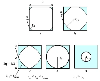
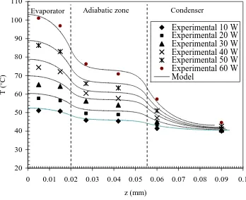
Theoretical and E xperimental Study on the Thermal Performance of F lat Miniature Heat Pipes Including Rectangular Grooves
by S. Maalej, J. Mansouri, M. B. H. Sassi, M. C. Zaghdoudi
266
E nhancement of Solar Thermal E nergy Storage Using Phase Change Materials: an E xperimental Study at Greek Climate Conditions
by Michalis Gr. Vrachopoulos, Maria K. Koukou, Dimitris G. Stavlas, Vasilis N. Stamatopoulos, Achilleas F. Gonidis, Eleftherios D. Kravvaritis
279
Thermal Modeling of Radiogenic Heating, Conduction, Melting, Metal-Silicate Segregation and Convection in Planetary Sciences
by S. Sahijpal
285
Analysis of Temperature F ield Inside the F uel Rod of the VVE R 440 F uel Assembly by Miriama Sačková, Branislav Hatala, Vladimír Nečas
291
Thermodynamic Analysis and Neural Network Model of Open Cycle Desiccant Cooling Systems with Silica Gel
by I. P. Koronaki, E. Rogdakis, T. Kakatsiou
298
Passive Control of the Turbulent F low Over a Surface-Mounted Rectangular Block Obstacle and a Rounded Rectangular Obstacle
by K. Aliane
305
Design Simulation of F iling Sequence and Solidification Time for Cast Metal Matrix Composite by Low Pressure Die Casting
by R. S. Taufik, S. Shamsuddin, K. K. Mak, A. A. Tajul, M. A. M. Khairul Anuar, B. B. T. Hang Tuah
315
Influence of Manufacturing Method and Interface Activators on the Anisotropic Thermal Behaviour of Copper Carbon Nanofibre Composites
by M. Kitzmantel, E. Neubauer, V. Brueser, M. Chirtoc, M. Attard
321
Thermal Diffusion Coating of Diamonds for Improved and Reliable Thermal Properties of Metal Diamond Composites
by M. Kitzmantel, E. Neubauer, I. Smid, C. Eisenmenger-Sittner, P. Angerer
325
Influence of Heat Transfer on the Thermomechanical Behavior of Shape Memory Alloys by Claire Morin, Ziad Moumni, Wael Zaki
329
Modeling and Simulation of Temperature Generated on Workpiece and Chip F ormation in Orthogonal Machining
by Hendri Yanda, Jaharah A. Ghani, Che Hassan Che Haron
340
Thermodynamic Analysis and E xperimental E valuation of Active and Passive Sorption Wheels by I. P. Koronaki, E. Rogdakis, T. Kakatsiou
349
E ffect of the Geometric Shape of the Roof (Type Habitat) on the Natural Convection with the Presence of a Heat Source
by E. Benachour, B. Draoui, L. Rahmani, B. Mebarki, L. Belloufa, K. Asnoune, B. Imine
355
Computational Study of the Conjugate Heat Transfer and the Wall Conduction E ffects in a Horizontal Pipe with Temperature Dependent Properties
by K. Chahboub, T. Boufendi
361
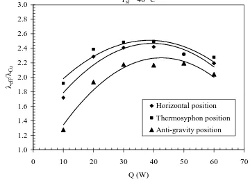
E xperimental Investigation of E lliptical Cross Section Geometry Wickless Heat Pipe Charged with Distilled Water and E thanol
by Ajit M. Kate, Ratnakar R. Kulkarni
International Review of Mechanical Engineering (I.RE.M.E.), Vol. 5, N. 2 Special Issue on Heat Transfer, February 2011
International Review of Mechanical Engineering (IREME)
Special Issue on Heat Transfer
Guest Editor-In-Chief
Alina Adriana Minea
Faculty of Materials Science and Engineering Technical University Gh. Asachi Iasi Bd. D. Mangeron no.59, Iasi, Romania
[email protected] [email protected]
Guest Editorial Board
Oronzio Manca
Dipartimento di Ingegneria Aerospaziale e Meccanica Seconda Università degli Studi di Napoli
Via Roma 29, Aversa (CE), Italy [email protected]
Harald Raupenstrauch
Department Metallurgy
Chair of Thermal Processing Technology University of Leoben
Franz Josef Strasse 18, Leoben, Austria [email protected]
Jennifer Wen
Director of Research, Faculty of Engineering Kingston University
Friars Avenue, Roehampton Vale, London [email protected]
International Review of Mechanical Engineering (I.RE.M.E.), Vol. 5, N. 2 Special Issue on Heat Transfer, February 2011
International Review of Mechanical Engineering (IREME)
Special Issue on Heat Transfer
Aim of the Special Issue
The aim of this special issue is to collect original research articles as well as review articles on the
most recent developments and research efforts in HEAT TRANSFER, with the purpose of
providing guidelines for future research directions.
Topics of interest include, but are not limited to:
•
Experimental techniques for measuring thermal properties
•
Conduction
•
Convection
•
Radiation
•
Combustion
•
Heat transfer applications
•
Heat transfer enhancement
•
Modeling of flow and heat transfer behavior of materials
International Review of Mechanical Engineering (I.RE.M.E.), Vol. 5, N. 2 Special Issue on Heat Transfer, February 2011
International Review of Mechanical Engineering (IREME)
Special Issue on Heat Transfer
Editorial
By the Guest Editor
HEAT TRANSFER area is very diverse in study methods and applications and that is making it
so challenging. Even if heat transfer, in some processes, is a secondary effect, knowledge in this
area is crucial for optimizing all the industrial processes and equipments and can interfere in final
economical situation.
As in previous years, a considerable effort has been devoted to research in traditional applications
such as chemical processing, general manufacturing, and energy conversion devices, including
general power systems, heat exchangers, and high performance gas turbines. In addition, a
significant number of papers address topics that are at the frontiers of both fundamental research
and important emerging technologies, including nanoscale structures, microchannel flows and basic
heat transfer.
There a lot of journals dedicated to Heat transfer in the market nowadays but on the other hand
there is a large number of research in this area.
Heat Transfer Special Issue on IREME provides a forum for research emphasizing
experimental work that enhances basic understanding of heat transfer and thermodynamics, and
their applications. In addition to the principal areas of research, the Special Issue covers research
results in related fields, including combined heat and mass transfer, micro and nanoscale systems,
multiphase flow, combustion, radiative transfer, porous media, cryogenics, turbulence, contact
resistance, and thermophysical property measurements and techniques.
The Heat Transfer Special Issue of IREME is to be seen as an instrument to enhance
interdisciplinarity and the discovery of new fields at the frontiers between different flavours of heat
transfer across the national boundaries.
Alina Adriana Minea
International Review of Mechanical Engineering (I.RE.M.E.), Vol. 5, N. 2 Special Issue on Heat Transfer, February 2011
Numerical Analysis of a Two-Dimensional Thermal Model
for a Car Under-Body
Antonio Di Micco
1, Francesco Fortunato
2, Oronzio Manca
1, Alina A. Minea
3, Daniele Ricci
1Abstract – In this paper a numerical bidimensional thermal analysis of the interactions between a car underbody and the road surface is carried out. The behaviour of the exhaust system and its thermal interface with the underbody is an important part of the thermal management of the car. In fact, the high value of temperatures along the exhaust system components such as catalytic converter, pipes, muffler determines strong thermal interaction with the other components close to the exhaust system. In order to preserve the more sensitive components and ensure safety and reliability, thermal shrouds are employed. Thermal design needs previous investigations on thermal and fluid dynamic behaviour by means of suitable numerical models and experimental measurements In this paper, the investigation is lead by means of the commercial code FLUENT on a model representing a section of the underbody near to the catalyst, the most critical component. The numerical analysis is carried out in laminar and transient state conditions, regarding the effects of natural convection in air and radiation. All thermo-physical properties of the fluid are assumed to be constant. Results are given in terms of temperature distributions, thermal and velocity fields considering several geometric parameters of the tunnel, such as the height, the distance from the road surface, the width and the length of the underbody. Copyright
© 2011 Praise Worthy Prize S.r.l. - All rights reserved.
Keywords:Natural Convection, Thermal Management, Thermal Design
Nomenclature
D Exhaust pipe diameter m
h Tunnel height m
H Distance from the road m
l Tunnel length m
k Thermal conductivity W m-1 K-1
L Under-body length m
Nu Nusselt number
q Heat flux W m-2
s Shield thickness m
t Time s
T Temperature K
x, y Spatial coordinate m
Greek Symbols
ε Emissivity
ν Kinematic viscosity m2 s-1
θ Dimensionless temperature
τ Dimensionless time
Subscripts
0 Initial condition
a Ambient
d Duct
f Fluid
I.
Introduction
The thermal management plays a fundamental role in the design and optimization of automotive systems [1],[2]. The high temperature values along the automotive exhaust systems components, such as catalytic converter, pipes, muffler and so on, determine critical thermal interaction with the other objects close to the exhaust system [3]. In this kind of problem the unknown variables are the heat transfer rates among the components and their temperatures [3]-[7]. The complex geometry of the exhaust line and the special flow conditions complicate the problem of accurately estimating several important heat transfer parameters.
Thermal design needs previous investigations on thermal and fluid dynamic behavior by means of suitable numerical models and experimental measurements, to detect the zones at higher temperatures. The heat transfer evaluation between the exhaust line, the underbody and the external ambient is needed [7]-[9].
Antonio Di Micco, Francesco Fortunato, Oronzio Manca, Alina A. Minea, Daniele Ricci
However, due to the high temperatures of the exhaust components and crowded engine compartment that may impede the external forced convection, one expects free convection heat transfer to be important, though along the external exhaust system in some stagnation zones buoyancy force could be significant.
In this paper a two-dimensional model of a section of the car underbody near to the catalyst, the most critical component belonging to the exhaust line [6], is proposed in order to study the interactions with the road surface and the exhaust system. The system is represented by a partially open horizontal cavity, heated by a duct placed in the middle. The vehicle is stationary so only the natural convection is regarded as well as the radiation mechanism.
Manca et al. [11] studied a configuration made of two horizontal parallel plates with the upper plate heated at uniform heat flux. Results were reported for Rayleigh numbers equal to 103 and 105 and for two aspect ratios.
Koca [12] provided a numerical study about the conjugate heat transfer in partially open square cavity with a vertical heat source for different Rayleigh numbers, conductivity ratios, opening position and open length. Jaluria et al. [13] provided a transient analysis of natural convection in air in a horizontal open ended cavity for a similar configuration and presented results for several significant variables, such as the penetration length, Rayleigh numbers and aspect ratio values.
In this work a transient analysis of the interaction of a car underbody with the exhaust system and the road surface is carried out in order to study the behavior of the system, with or without thermal shields. The vehicle is assumed to be stationary so natural convection is the primary heat transfer mode.
II.
Description of the Geometrical and
Numerical Model
The numerical model is a two-dimensional model of a car underbody section, close to the catalyst, interacting with the road surface and the exhaust line. In order to study the influence of the introduction of the thermal shields, a numerical model is developed. Figure 1(a) shows the considered geometric parameters, such as L, the under-body length, l, the tunnel length, H, the distance from the road surface, h, the tunnel height and
D, the pipe diameter. As shown in Figure 1(b), the exhaust pipe warms up the underbody wall, because its temperature is set to 873 K and air comes in and out the channel by the bottom side walls IN/OUT. The numerical analysis is carried out in laminar and transient state conditions. The considered fluid is air and all the thermo-physical properties are assumed to be constant, except for the dependence of density on the temperature (Boussinesq approximation) which gives rise to the buoyancy forces. Temperature is evaluated at an average temperature calculated between the exhaust system value and ambient one (Ta = 300 K).
(a)
(b)
Figs. 1. (a) sketch of the model and geometric parameters; (b) model including thermal shields
The investigation is accomplished by means of FLUENT code [14]. As the car is assumed to be stationary, the main heat transfer mechanism is represented by natural convection. However, radiative effects are taken into account and the emissivity of the thermal shield is set to 0.13 while their thickness and thermal conductivity are equal to 0.7x10⁻³ m and 200 W/mK, respectively. The temperature of road surface is 333 K. The exhaust system pipe diameter is 0.04 m and its emissivity is 0.85 while ε for the underbody and road is 0.98 and 0.90, respectively. The base configuration of the model is characterized by H = 0.12 m, L = 0.85 m, l/h
= 2.27 while the other geometric ratios and parameters considered in the investigation are shown in Table I.
TABLE I
GEOMETRIC PARAMETERS CONSIDERED IN THE INVESTIGATION
l/h H [m] L [m]
1.00 0.09 0.60
1.45 0.12 0.70
2.00 0.15 0.85
2.27 0.24 0.90
3.26 0.36 1.00
4.00
Antonio Di Micco, Francesco Fortunato, Oronzio Manca, Alina A. Minea, Daniele Ricci
= 300 K. The effects of radiation are taken into account, too. The Discrete Transfer Radiation Model (DTRM) is employed, assuming all surfaces to be diffuse. A grid independence analysis has been lead in order to individuate the best compromise between the accuracy and computational time.
Four different non-structured meshes have been developed considering the model characterized by l = 0.250 m, h = 0.110 m, H = 0.120 m and L = 0.850 m without thermal shields. They have a number of nodes equal to 10676, 17194, 25206 and 41802, respectively. The third mesh has been adopted because the comparison of the results in terms of tunnel and side wall temperatures with a coarsen mesh has revealed a little difference, at most equal to 0.15% as shown in Figure 2.
Furthermore, a sensitivity analysis of the solution on the time step have been accomplished, choosing a value equal to 0.2 s, and several simulations have been carried out to set properly the radiation model parameters. Results are presented in terms of dimensionless parameters, defined by the next relations:
(
0)
.
d f
qD Nu
T T k
=
− (1)
0
0
d
T T T T θ= −
− (2)
2
t D
ν
τ = (3)
t [s]
T[
K
]
10 20 30 40 50
340 360 380 400 420 440 460 480 500 520
Model 1 Model 2 Model 3 Model 4
Fig. 2. Temperature profiles of the tunnel walls depending on time for the four considered mesh grids
III.
Results and Discussion
Results for the transient analysis are given in order to study the influence about the main geometric parameters on the heat transfer interaction for a car under-body with the exhaust system and road surface. Several
characteristic ratios for l/h have been studied such as 1.00, 1.45, 2.00, 2.27, 3.26 and 4.00 and for the base configuration the behaviour depending on H and L has been investigated. The results are presented in terms of dimensionless variables. Figure 3 depicts the Nusselt number profiles depending on dimensionless time for the configurations without thermal shields and for different
l/h ratios. It is observed that Nu decreases as this geometric ratio increases. In fact, for l/h = 1.00 Nu is equal to 48 when the steady state condition is reached while for l/h = 4.00 Nu augments about 20% because the distance between the exhaust system and the under-body is reduced. Moreover, the steady state condition is observed for growing times as l/h decreases.
τ
Nu
0.5 1 1.5
50 55 60 65 70
l/h = 1.00 l/h = 1.46 l/h = 2.00 l/h = 2.27 l/h = 3.26 l/h = 4.00
Without Thermal Shield
Fig. 3. Nusselt number profiles depending on dimensionless time for different l/h ratios without thermal shields
Figures 4 present the results in terms of average dimensionless temperature of the tunnel surface depending on time for different l/h ratios. Figure 4(a) is referred to the configurations without thermal shields and show that the lower is the l/h the higher are the average temperatures. The introduction of the thermal shields reduces the temperatures and this behaviour is more evident as l/h augments, as depicted in Fig. 4(b). At l/h = 2.27 a decrease equal to 6% is detected.
Because the vehicle is stationary the heat transfer mechanism is due to natural convection together with the radiation.
The exhaust system warms up the surrounding air and the fluid moves up towards the tunnel only because density changes.
In this way, a thermal plume develops and rises from the duct creating two different branches.
Two convective cells are detected and the temperature and velocity fields are influenced by the introduction of the thermal shields and by the geometric ratios (Figs. 5-6).
Antonio Di Micco, Francesco Fortunato, Oronzio Manca, Alina A. Minea, Daniele Ricci
τ
θ
0.5 1 1.5
0.2 0.3 0.4 0.5 0.6 0.7
l/h = 1.00 l/h = 1.46 l/h = 2.00 l/h = 2.27 l/h = 3.26 l/h = 4.00
Without Thermal Shield
(a)
τ
θ
0.5 1 1.5
0.1 0.2 0.3 0.4 0.5 0.6 0.7
l/h = 1.00 l/h = 1.46 l/h = 2.00 l/h = 2.27 l/h = 3.26 l/h = 4.00
With Thermal Shield
(b)
Figs. 4. Average dimensionless temperature profiles of tunnel surface depending on time for different l/h ratios: a) without thermal shields; b)
with thermal shields (s = 0.007 m)
The fluid flow may be choked for the effect of the mutual positions of duct and surrounding surfaces and the heat transfer becomes less efficient.
Moreover, the radiation works parallel to the natural convection and the heat transfer is more efficient when the duct reaches for the tunnel surfaces.
Fig. 5. Temperature fields at the steady state condition: a) l/h = 2.27, H
= 0.12 m and L = 0.85 m
Fig. 6. Stream functions contours at the steady state condition: a) l/h = 2.27, H = 0.12 m and L = 0.85 m
Figures 7 show a similar behaviour regarding the average temperatures on the tunnel side walls as the l/h
ratio changes. In fact, for l/h = 2.27 a reduction of 10% is evaluated by introducing the thermal shields. Temperatures are generally lower than ones calculated for the tunnel roof because the side walls are not directly exposed to the thermal plume rising from the exhaust system.
τ
θ
0.5 1 1.5
0.1 0.2 0.3 0.4 0.5 0.6 0.7
l/h = 1.00 l/h = 1.46 l/h = 2.00 l/h = 2.27 l/h = 3.26 l/h = 4.00
With Thermal Shield
(a)
τ
θ
0.5 1 1.5
0.2 0.3 0.4 0.5 0.6 0.7
l/h = 1.00 l/h = 1.46 l/h = 2.00 l/h = 2.27 l/h = 3.26 l/h = 4.00
Without Thermal Shield
(b)
Figs. 7. Average dimensionless temperature transient profiles of tunnel side surface for different l/h ratios: a) without thermal shields; b) with
Antonio Di Micco, Francesco Fortunato, Oronzio Manca, Alina A. Minea, Daniele Ricci
Figure 8 depicts the temperature distribution along the tunnel roof wall when steady state condition is reached. For small l/h ratios the temperature distribution are more homogeneous, the radiation effect are less evident and the detected temperatures are the highest. When l/h raises the distance between surfaces and duct reduces and the central part of the roof walls is heated by radiation, significantly. The introduction of the thermal shield decreases the temperature values and distribution are more homogeneous.
x / l
θ
0 0.25 0.5 0.75 1
1.4 1.45 1.5 1.55 1.6 1.65
l/h = 1.00 l/h = 1.46 l/h = 2.00 l/h = 2.27 l/h = 3.26 l/h = 4.00
With Thermal Shield
Fig. 8. Temperature profiles of tunnel roof surface for different l/h at steady state condition with thermal shields
In Figure 9 results are presented in terms of average dimensionless temperature of the tunnel side walls for different l/h ratios and investigate the influence of the thermal shields.
As described, the introduction of the thermal shield tends to decrease the temperatures evaluated on the tunnel side walls and this behavior is more evident as l/h
augments.
y / h
θ
0 0.25 0.5 0.75 1
1.1 1.2 1.3 1.4 1.5 1.6
l/h = 1.00 l/h = 1.46 l/h = 2.00 l/h = 2.27 l/h = 3.26 l/h = 4.00
With Thermal Shield
Fig. 9. Dimensionless temperature profiles of tunnel side surface for different l/h ratios at steady state condition for the configuration with
thermal shields (s = 0.007 m)
Figure 10 shows the Nusselt number profile depending on time for the base configuration with thermal shields for different values of the underbody total width, L. Nusselt number raises as L decreases although differences are not so significant.
In this way, it is possible to focus the attention on simpler models characterized by small L and reduce computational times.
τ
Nu
1 2
55 60 65 70
Ltot= 0.60 m
Ltot= 0.70 m
Ltot= 0.85 m
Ltot= 0.90 m
Ltot= 1.00 m
With Thermal Shield
Fig. 10. Nusselt number profile depending on time for the base configuration with thermal shields for different values of L
Figures 11 are referred to the base configuration characterized by l/h = 2.27 with thermal shields and describes the behaviour of the system by changing the distance of the under-body from the road surface. Figure 10(a) depicts the Nusselt number profiles for different values of H. It is observed that for the largest value of H
the steady state condition is not reached.
Nu rises as H grows although differences are not much evident.
The steady state condition, moreover, is detected for larger dimensionless times as H augments.
Figure 11(b) presents the results in terms of temperature distribution along the tunnel roof wall.
From the figure it is easy to observe two relative maximum. This behaviour is related to presence of the convective cells rising from the heated duct. The maximum values are attained at x/l = 0.3 and 0.7, respectively and profiles are perfectly symmetric.
The highest maximum values of dimensionless temperature are detected for H = 0.009 m because the fluid flows difficultly in the tunnel and in correspondence of the inlet and outlet sections.
The minimum value of the dimensionless temperature is detected at x/l = 0.5.
IV.
Conclusion
Antonio Di Micco, Francesco Fortunato, Oronzio Manca, Alina A. Minea, Daniele Ricci
τ
Nu
1 2
55 60 65 70
H = 90 x 10-3
m H = 120 x 10-3
m H = 150 x 10-3
m H = 240 x 10-3
m H = 360 x 10-3
m
With Thermal Shield
(a)
x / l
θ
0 0.25 0.5 0.75 1 1.485
1.49 1.495 1.5 1.505 1.51 1.515 1.52
H = 90 x 10-3
m H = 120 x 10-3
m H = 150 x 10-3
m H = 240 x 10-3
m H = 360 x 10-3m
With Thermal Shield
(b)
Figs. 11. Influence of the distance from the road surface, H: a) Nusselt numbers profile depending on time; b) temperature distribution along
the tunnel roof surface at the steady state condition
The model represents the section close to the catalyst component and the interaction of the underbody with the exhaust system, represented by a heated duct, and the road surface was investigated by changing different aspect ratios.
The under-body problem was solved by means of FLUENT. Results showed that Nusselt number increases as l/h ratio and H rise. The introduction of the thermal shields above the exhaust system reduces the calculated average temperatures and this effect is more significant for larger l/h ratios; the steady state condition is detected for larger times. The temperature of the tunnel roof surface and side walls augments as l/h and H decrease and for H = 0.36 m the steady state condition is not observed.
Acknowledgements
This work was supported by a Legge 5 Regione Campania grant.
References
[1] P. Setlur, J. Wagner, D. Dawson and E.E. Marotta, An advanced engine thermal management system: nonlinear control and test, IEEE/ASME Transactions on Mechatronics, vol. 10, pp. 210-220, 2005.
[2] J. Wagner, I. Paradis, E. Marotta, and D. Dawson, Enhanced Automotive Engine Cooling Systems-A Mechatronics Approach for Thermal Efficiency Gains, Mechatronics in Automotive Systems-International Journal of Vehicle Design, 28, No. 1/2/3, pp. 214-240, 2002.
[3] P.A. Battiston, A. Alkidas and D.J. Kapparos, Temperature and Heat Transfer Measurements in the Exhaust System of a Diesel-Powered Light Duty Vehicle, 2003 Vehicle Thermal Management Systems Conference Proceedings, IMechE Paper C599/100/2003, VTMS 6 Conf. Proc., pp. 485-510, 2003.
[4] F. Fortunato, F. Damiano, L. Di Matteo and P. Oliva, Il supporto dell’analisi virtuale nella predizione dei flussi termici nel sottocofano di un veicolo, Rivista dell’ATA, vol. 58, n. 7/8, pp. 120-125, 2005.
[5] F. Fortunato, A. Giaquinto, O. Manca, S. Nardini and F. Quadrini, Analisi termica bidimensionale dell’influenza degli schermi radiativi sullo scarico di un autoveicolo, Atti del XXIV Congresso Nazionale UIT, pp. 531-536, Napoli, 21-23 giugno, 2006, ETS Pisa 2006.
[6] D. J. Kapparos, D. E. Foster and C. J. Rutland, Sensitivity Analysis of a Diesel Exhaust System Thermal Model, SAE Paper 2004-01-1131, 2004.
[7] F. Fortunato, M. Caprio, P. Oliva, G. D'Aniello, P. Pantaleone, A. Andreozzi and O. Manca, Numerical and Experimental Investigation of the Thermal Behavior of a Complete Exhaust System, SAE Paper 2007-01-1094, 2007.
[8] A. C. Alkidas, P. A. Battiston and D. J. Kapparos, Thermal Studies in the Exhaust System of a Diesel-Powered Light-Duty Vehicle, SAE Paper 2004-01-0050, 2004.
[9] P. J. Shayler, D. J. Hayden and T. Ma, Exhaust System Heat Transfer and Catalytic Converter Performance, SAE Paper 1999-01-0453, 1999..
[10] P. Kandylas and A. M. Stamatelos, Engine Exhaust System Design Based on Heat Transfer Computation, Energy Conversion & Management, vol. 40, pp. 1057-1072, 1999.
[11] A. Andreozzi, O. Manca, B. Morrone, Numerical Analysis of Natural Convection in Air in a Horizontal Open Ended Cavity Uniformly Heated from the Upper Plate, Proc. of the National Heat Transfer Conference, vol. 2, pp. 1519-1527, 2001.
[12] A. Koca, Numerical Analysis of Conjugate Heat Transfer in a Partially Open Square Cavity with a Vertical Heat Source, International Communications in Heat and Mass Transfer, vol. 35 (10), pp. 1385-1395, 2008.
[13] A. Andreozzi, O. Manca, Y. Jaluria, Transient Analysis of Natural Convection in a Horizontal Open Ended Cavity, ASME Heat Transfer Division, vol. 372 (1), pp. 135-146, 2002.
[14] Fluent v6.4 user guide, Fluent Corporation, 2006
Authors’ information
1Dipartimento di Ingegneria Aerospaziale e Meccanica, Seconda
Università degli Studi di Napoli, via Roma 29, 81031 Aversa, Italy.
2Elasis S.C.p.A. –
FPT, via Ex Aeroporto, 80038 Pomigliano d’Arco – Italy.
3Department of Plastical Processes and Heat Treatment,
International Review of Mechanical Engineering (I.RE.M.E.), Vol. 5, N. 2 Special Issue on Heat Transfer, February 2011
Optimization of Turbulence and Radiation Models
for an Improved Prediction of Non-Premixed Turbulent Flames
C. Pfeiler, C. J. Spijker, H. Raupenstrauch
Abstract – Turbulent combustion of gaseous fuels is of importance especially for the steel industry. To predict details on the concentration fields, an accurate modeling of turbulence and temperature is required. If industrial scale combustion has to be predicted, the dimension of the geometry leads to a limit of models that can be used efficiently. Therefore, an optimization of turbulence and radiation models has been performed. The accuracy of the realizable k-epsilon and the Reynolds Stress model (RSM) for the turbulence and the Discrete Transfer Radiation Model (DTRM) and the Discrete Ordinate model (DO) for radiation are compared. The combustion system is a non-premixed diluted methane flame (Sandia flame D). The stationary laminar flamelet model together with the GRI-Mech 3.0 mechanism was applied. A modification
of the empirical turbulence model constant C2 helped to get better correlation with the
experimental data. The DO radiation model, applying fewer rays, gives similar but faster results
than the DTRM model. Copyright © 2011 Praise Worthy Prize S.r.l. - All rights reserved.
Keywords:Burner, Combustion, Flamelet, Radiation, Sandia Flame D, Turbulence
I.
Introduction
For a detailed prediction of turbulent flames, computational intensive models such as the Composition PDF Transport combustion model or the Large Eddy Simulation (LES) model for the turbulence are used [1]. Composition PDF Transport Models allow accurate predictions especially for kinetically controlled species such as NO or CO. It is mainly used for detailed studies on flames including ignition or extinction phenomena. Even if an ISAT algorithm is used, the model is computationally intensive [2], [3]. The combination of the PDF Transport combustion model and the LES turbulence model, which directly solves large scale eddies and uses sub-grid turbulence models for smaller scales, is ideal for studying detailed flame phenomena. A subgrid-scale model for LES was recently combined together with the Eddy Dissipation Concept combustion model to model the non-premixed “Sandia Flame D” [4].
For industrial applications, LES can be used e.g. for studying transient flow phenomena, but without considering combustion.
To study only the flow, a high performance computing system is already necessary. For an optimization of furnaces, burners and processes, like reheating of slabs or in-situ burning of process gases and dusts, the modeling of combustion is of crucial importance. It would be ideal to have the opportunity to predict combustion processes using those advanced models also for industrial scales within an adequate computation time.
C. Pfeiler, C. J. Spijker, H. Raupenstrauch
II.
Model Description
Mass and momentum conservation in the computational domain were achieved by solving the continuity equation and the Navier Stokes equations for Newtonian fluids. The solution yields the pressure and velocity components at every point in the 2D and 3D domain. The solution of the flow and the mixing field is performed in ANSYS Fluent, a Computational Fluid Dynamics code, with the Stationary Laminar Flamelet Model (SLFM) used for chemistry [8]. The turbulent flow field was modeled with the realizable k-ε and the Reynolds Stress Model (RSM). To account for radiation the Discrete Transfer Radiation Model (DTRM) and the Discrete Ordinates (DO) model are evaluated.
II.1. Stationary Laminar Flamelet Model (SLFM)
The Flamelet model is a method to combine detailed chemical reactions and turbulent flow within moderate computational time. It is based on the assumption, that the turbulent non-premixed flame is composed of a multitude of one-dimensional discrete laminar counter-flow diffusion flames called flamelets. As the velocity of the counter flowing jets increase, the flame is strained and increasingly departs from chemical equilibrium. The governing equations can be simplified to one dimension along the axis of the fuel and oxidizer jets. In that one dimension complex chemistry calculations can be performed. The width of these flamelets is assumed to be smaller than the Kolmogorov scale, which separates combustion and turbulence at different scales [9]. It is assumed that the pressure is constant and the Lewis number for all the species is unity. The flamelet equations are derived applying a coordinate transformation with the mixture fraction as an independent coordinate to the governing equations for the temperature, T, and the species mass fractions, Yi,
[10]: 2 2 1 1 2 1 2 rad i i
p i p
p i p ,i p i q T T H S
t Z c c
c Y T
c
c Z Z Z
ρ ρχ ρχ ∂ = ∂ − + + ∂ ∂ ∂ ⎡ ∂ ⎤∂ + ⎢∂ + ∂ ⎥∂ ⎣ ⎦
∑
∑
(1)2 2 1 2 i i i Y Y S t Z ρ∂∂ = ρχ∂ +
∂ (2)
Here, ρ is the density, cp,iand cp are the ith species
specific heat capacity and mixture-averaged specific heat, respectively. t is the time, Z the mixture fraction, Si
the species reaction rate, Hi the specific enthalpy, qrad the
radiation source/sink term and χ is the scalar dissipation rate.
Instead of using the strain rate, as =v 2d, to quantify the departure from equilibrium, the scalar dissipation is
used. v describes the relative velocity of the fuel and oxidizer jets and d is the distance between the jet nozzles. The scalar dissipation rate is modeled across the flamelet. To include the effect of density variation, the modeling of the scalar dissipation is based on [11]:
( )
(
)
( )
2 2 1 3 14 2 1
2 erfc 2
s a Z exp Z ρ ρ χ π ρ ρ ∞ ∞ − + = ⋅ + ⎛ ⎡ ⎤ ⎞ ⋅ ⎜− ⎣ ⎦ ⎟ ⎝ ⎠ (3)
where ρ∞ is the density of the oxidizer stream, as is the
characteristic flamelet strain rate and erfc-1 is the inverse complementary error function. However, the scalar dissipation varies along the axis of the flamelet. For a counterflow geometry the flamelet strain rate, as, can be
related to the scalar dissipation at the position where the mixture fraction, Z, is stoichiometric. The following parameterized scalar dissipation rate is used:
( )
( )
( )
(
)
2 1 2 12 erfc 2
2 erfc 2
st st exp Z Z Z exp Z χ χ − − ⎛− ⎡ ⎤ ⎞ ⎜ ⎣ ⎦ ⎟ ⎝ ⎠ = ⎛− ⎡ ⎤ ⎞ ⎜ ⎣ ⎦ ⎟ ⎝ ⎠ (4)
The value of the stoichiometric scalar dissipation rate parameter χst must cover the range from equilibrium to
extinction.
The advantage of reducing the complex chemistry to two variables allows the flamelet calculations to be pre-processed, which makes the simulation faster. It is assumed that the flame respond immediately to the aerodynamic strain. Therefore, the model cannot capture deep non-equilibrium effects e.g. slow chemistry or ignition.
During the flow field calculation the conservation equations for the mean mixture fraction, Z , and its variance, Z "2 , describe the mixing of fuel and oxidizer. The assumption of equal diffusivity in turbulent flow reduces the species equations to a single mixture fraction equation. The Favre-averaged mixture fraction and mixture fraction variance equations are [12]:
( ) ( )
tZ
Z uZ Z
t Sc
µ
ρ ρ ⎛ ⎞
∂ + ∇⋅ = ∇⋅ ∇
⎜ ⎟
∂ ⎝ ⎠ (5)
( ) ( )
( )
2
2 2 2
2
2 2
2 86 2
t
Z "
t
Z " u Z " Z "
t Sc
. Z " Z "
k µ ρ ρ ε µ ρ ⎛ ⎞ ∂ + ∇⋅ = ∇⋅⎜ ∇ ⎟+ ⎜ ⎟ ∂ ⎝ ⎠ + ∇ − (6)
C. Pfeiler, C. J. Spijker, H. Raupenstrauch
Here, ScZand 2
Z"
Sc are the Schmidt numbers and are chosen to be 0.85. µt is the turbulent viscosity, k is the turbulence kinetic energy and ε is its dissipation rate. Z is assumed to follow, p, the presumed β-function PDF [13]. The mean values of mass fractions of species, temperature and density, presented as φ can be calculated, in non-adiabatic systems assuming enthalpy fluctuations independent from the enthalpy level as:
( )
( )
1
0
Z ,H p Z dZ
φ =
∫
φ (7)where, H is the mean enthalpy which is defined as:
( ) ( )
th p
k
H uH H S
t ρ ρ c
⎛ ⎞
∂ + ∇⋅ = ∇⋅⎜ ∇ ⎟+
⎜ ⎟
∂ ⎝ ⎠ (8)
Here, Sh is a sink or source term due to radiation or heat
transfer to wall boundaries.
II.2. Realizable k- ε Turbulence Model
To predict an accurate spreading rate of round jets the realizable k-ε model is a good opportunity. The Boussinesq approach of this model assumes the turbulent viscosity as an isotropic scalar quantity. The advantage of this approach is the relatively low computational cost, although the isotropic assumption is not valid for most of the turbulent flows. The model includes an eddy-viscosity formula and a model equation for dissipation [14]. The equation for the turbulent kinetic energy is the same as that in the standard k-ε model. The dissipation equation is based on the dynamic equation of the mean-square vorticity fluctuation. Cµ is computed as a function
of k and ε. The model constants C2 = 1.9, σk = 1.0, and
σε = 1.2 have been established to ensure that the model
performs well for certain canonical flows [13]. In this work for some results the standard value of the model constant C2 was changed to C2 = 1.8 as recommended in
literature for the standard k- ε model [15].
II.3. Reynolds Stress Turbulence Model (RSM)
Measurements on the Sandia flame D show anisotropic turbulent fluctuations [16]. Compared to the k-ε model the Reynolds stress model is able to account for anisotropic turbulent flows. It solves a transport equation for each of the stress terms in the Reynolds stress tensor. RSM is better for situations in which the anisotropy of turbulence has a dominant effect on the mean flow. Since in 3D seven additional transport equations have to be solved, this turbulence model is more computational intensive as the realizable k- ε model.
II.4. Discrete Transfer Radiation Model (DTRM)
The model assumes the radiation leaving a surface element, in a certain range of solid angles, can be approximated by a single ray. Optical refraction and scattering effects are neglected. The change of radiation intensity I along the path s is defined as:
4
B
a T
dI aI ds
σ π
+ = (9)
where, a is the absorption coefficient, σB the
Stefan-Boltzmann constant which is σB = 5.672e-08 W/m²K4, I
is the radiation intensity and T the local temperature. Eq. (9) is integrated along a series of rays emanating from boundary faces. To achieve accurate results a high number of rays is necessary. This causes long computation times.
II.5. Discrete Ordinates Radiation Model (DO)
The DO model uses transport equations for radiation intensity. It solves for as many transport equations as there are directions, s. In contrast to the DTRM model, the DO model includes reflection, refraction and scattering. The position vector, r, accounts for the radial spreading of rays. Thus, fewer discrete rays are required. The radiation intensity is written as [17]:
( ) (
) ( )
( ) (
)
4 2
4
0 4
B s
s
dI r ,s T
a I r ,s an
ds
I r ,s s s ' d '
π
σ
σ π
σ π
+ + = +
+
∫
Φ ⋅ Ω(10)
where, s 'is the standardized direction vector of the scattered radiation, σs is the scattering coefficient, n is the
refraction index, Φ is the phase function for the scattered radiation and Ω' is the solid angle to the solid wall. In both radiation models the absorption coefficient, a, is determined by the Weighted Sum of Grey Gases (WSGGM) Model. Here, a is a function of local concentrations of CO2 and H2O-vapor and is
defined as [18]:
b i i
a=
∑
b p (11)Here, bb are polynomials and piis the partial pressure
of the ith species.
III.
Experimental Data
C. Pfeiler, C. J. Spijker, H. Raupenstrauch
Darmstadt in Germany [15], [16]. The experimental and simulation conditions are shown in Table I.
TABLEI
EXPERIMENTAL AND SIMULATION CONDITIONS [15],[16]
Jet diameter [m] 0.0072
Pilot diameter [m] 0.0182
Jet composition CH4/air [vol.-%] 25/75
Pilot mixture fraction [-] 0.27
Jet Reynolds number [-] 22,400
Jet velocity [m/s] profile
Pilot velocity [m/s] profile
CO flowing air velocity [m/s] 0.9
Relative velocity jet-co flow[m/s] 48.7
Fuel temperature [K] 294
CO flowing air temperature [K] 291
Methane is partially premixed with air to prevent almost completely soot formation and to provide a stable flow field. However, this flame burns as a non-premixed flame with a single reaction zone near the stoichiometric mixture. In fuel rich regions significant premixed reactions were not observed [16]. The Reynolds number of the jet exit is 22,400 with a low probability of localized flame extinction. The pilot flame burns a mixture of gases having the same composition and enthalpy as a CH4/air mixture at 0.27 mixture fraction. A
coflowing air was placed around the flame to avoid the influence of airflow in radial direction. The coflowing air parallel to the flame was about 0.9 m/s.
IV.
Simulation Details
2D axisymmetrical and 3D simulations are performed. The burner is positioned in the center of the coflowing air as shown in Fig. 1.
The distance between the burner center and the domain border is chosen to be 0.036 m to minimize the influence of the boundary condition there. Details of the burner nozzle are given in Fig. 2.
The computational domains are discretized into hexahedral elements that are refined around the inlet of the burner nozzle.
The 2D grid consists of 11970 elements and the 3D grid of 228,800 elements.
Fig. 1. 3D geometry with the burner in the center of the of the coflowing air region. Units are given in [mm]
Fig. 2. Details of the piloted burner nozzle. Units are given in [mm]
A mesh sensitivity analysis was performed only for the 2D simulations [19]. The mesh was optimized in axial direction regarding the mixture fraction and in radial direction regarding the axial velocity. The 2D grid is shown in Fig. 3.
C. Pfeiler, C. J. Spijker, H. Raupenstrauch
In order to get an equivalent comparison, the 3D grid elements are distributed in the same way as for the 2D grid. The inlet velocity profile for the pilot and burner is positioned at the exit plane of the burner.
Inlet turbulence parameters for k and ε were either estimated values, constant or linearized values based on measurements [16]. At the outlet, the surface surrounding the co-flowing air and the surface opposite of the burner, a constant pressure is applied as boundary condition. Material and process data used for the simulations are summarized in Table I. The equations are solved using the ANSYS-FLUENT CFD package. The thermo physical data of FLUENT are used. To account for detailed chemical kinetic the Gri-Mech 3.0 mechanism was implemented, considering 53 species and 325 reactions [20].
For all simulations presented in this paper, a second order upwind scheme was used for the conservation equation of momentum, turbulent kinetic energy, turbulent dissipation rate, mean mixture fraction and mean mixture fraction variance. The Presto scheme was used for interpolation methods for pressure [13]. Simple was chosen for the coupling between velocity and pressure [13].
V.
Results and Discussions
In the present study, the stationary laminar flamelet approach is applied and the turbulence flow field for the Sandia Flame D is predicted with the realizable k-ε model in 2D case and RSM in a 3D case. The effect of the assumption of isotropic turbulence predicted with the k- ε model and the possibility of an anisotropic turbulence calculation with RSM as well as the change of the empirical turbulence constant C2 are studied. The
effect of radiation is studied using the DTRM and the DO radiation model. The results are compared to experimental data [15], [16].
In most cases, inlet values for k and ε have to be estimated.
For the Sandia Flame D measurements of the turbulent kinetic energy profile at the burner exit (inlet of the simulation domain) is available.
A short study has been performed to show the effect on the flame temperature with various turbulence inlet conditions. The conditions have been chosen as an estimated value (turbulent intensity of 10 %), as a constant value (mean value of k from the measured profile) and as a linearized profile of the measured turbulent kinetic energy.
The effect of different turbulence inlet boundary conditions is shown in Fig. 4.
Here, the temperature along the center line of the flame is compared. In the case of the estimated values, the predicted temperature is farthest from the experimental data.
The constant value and linearized profile based on measurements show better agreement, mainly in the near region of the burner.
Both of them give similar results. In this simulation, radiation was neglected and the realizable k- ε was chosen as turbulence model.
0 500 1000 1500 2000
0 20 40 60 80 100
x/d[-]
T
em
p
era
ture
[
K
]
Experimental Data; C2 = 1.9 Estimated Value; C2 = 1.9 Constant Value; C2 = 1.9 Linearized Profile; C2 = 1.9
Fig. 4. Comparison of the axial temperature profiles with experimental data for different turbulence boundary conditions [15]. Here, x is the axial distance from the burner nozzle and d is the diameter of the nozzle
Fig. 5. Predicted temperature field for the Sandia Flame D in 2D axisymmetric
It seems that a constant value for k and ε as inlet condition is adequate, but it has to be selected carefully. The predicted temperature field of the flame in 2D axisymmetric is shown in Fig. 5. A comparison of the axial temperature is given in Fig. 6. Radiation is not considered in this case. Realizable k- ε gives a slightly lower maximum temperature than RSM.
Measurements have shown anisotropic turbulence in this flame [16].
The estimation, that the consideration of the known anisotropic turbulence in this flame with the RSM model can reproduce the measured temperatures, was not achieved. Both models, realizable k- ε and RSM with standard turbulence constants, were not able to reproduce the measurements exactly. The change of the proposed turbulence constant C2 for both turbulence models to a
value of C2 = 1.8, produces a change in the axial
temperature curve as can be seen in Fig. 6.
The value of C2 was recommended for the standard k-
ε model [15].
However, for the realizable k-ε and RSM it seems to have an important effect on a better prediction of turbulent non-premixed jet flames as well.
C. Pfeiler, C. J. Spijker, H. Raupenstrauch
predict the measurement data better until the position x/d = 50. Subsequently, the decline of temperature is lower than in the experiment.
These results demonstrate that realizable k-ε in 2D and RSM in 3D, with the turbulence constant C2 = 1.8, are
able to predict the flame temperature more accurate as using the standard turbulence constants.
Fig. 6. Comparison of the axial temperature profiles with experimental data [15]. Here, x is the axial distance from the burner nozzle and d is
the diameter of the nozzle
The reason for the effect of changing the turbulence constant C2 is shown in Fig. 7. The simulations using the
standard turbulence parameters over-predict the turbulent kinetic energy in the flame center. A decrease of C2 in
both cases decreases the maximum of the curve. Also a slight shift to the right can be observed. C2 is a factor for
a sink in the turbulence dissipation equation. A decrease of that factor leads to a lower reduction of dissipation and a faster reduction of turbulent kinetic energy. Thus, C2 is the amount of lost rotational energy due to friction.
The mixing of fuel and oxidizer is strongly coupled with turbulence. The lower turbulence decreases the mixing of methane and air. Therefore, the consumption of methane is slower. Representatively, the distribution of mass fraction of methane along the centerline is shown in Fig. 8. The results of all simulations which has been performed show a faster decrease of methane mass fractions in comparison to the measurements. The fastest consumption of methane occurs with the predictions by the use of the standard values for C2 = 1.9 and C2 = 1.92
for realizable k- ε or RSM, respectively. The complete methane concentration is consumed at the position x/d = 40. The experimental data and the simulations with C2 = 1.8 show the total consumption at the position of
x/d = 50.
The radial profiles of temperature at the position x/d = 45 have the same tendency as the axial profiles. By changing the turbulence constant, the predicted curves agree better with the measurement data (Fig. 9). However, the accordance is less than that for the axial profiles. The calculations predict a later temperature decay along the radial position x/d = 45. In case of C2 = 1.8 the decline is the same as that for the
measurements. In contrast, the predicted curves with standard values for the turbulence constants, the decrease in temperature is lower.
It has to be mentioned that due to the axial shifted temperature peak (Fig. 6), the predicted temperature at the axis is lower than experimental data show at this position.
To account for radiation, two models have been evaluated.
The Discrete Transfer Radiation Model (DTRM) and the Discrete Ordinates Model (DO). In this evaluation the 2D axisymmetrical domain together with the realizable turbulence model are used.
To achieve accurate results with the DTRM model a high number of rays in Phi and Theta direction are necessary.
0 20 40 60 80
0 20 40 60 80 100
T
u
rb
ki
ne
ti
c
en
er
g
y
[m
²/
s²
]
x/d [-]
Experimental Data
2D realizable k-epsilon, C2 = 1.9 2D realizable k-epsilon, C2 = 1.8 3D RSM, C2 = 1.92 3D RSM, C2 = 1.8
Fig. 7. Axial turbulent kinetic energy profiles compared with experimental data [16]. Here, x is the axial distance from the burner
nozzle and d is the diameter of the nozzle
0.00 0.05 0.10 0.15
0 10 20 30 40 50 60
CH
4
M
as
s F
ra
ct
ion
[-]
x/d [-]
Experimental Data
2D realizable k-epsilon, C2 = 1.9 2D realizable k-epsilon, C2 = 1.8 3D RSM, C2 = 1.92 3D RSM, C2 = 1.8
Fig. 8. Axial methane mass fraction compared with experimental data [15]. Here, x is the axial distance from the burner nozzle and d is the
diameter of the nozzle
0 500 1000 1500 2000
0 2 4 6 8 10
T
em
p
er
at
u
re
[
K
]
r/d [-]
Experimental Data
2D realizable k-epsilon, C2 = 1.9 2D realizable k-epsilon, C2 = 1.8 3D RSM, C2 = 1.92 3D RSM, C2 = 1.8
Fig. 9. Radial temperature profiles at x/d = 45 compared with experimental data [15]. Here, r is the distance in radial direction and d
C. Pfeiler, C. J. Spijker, H. Raupenstrauch
This leads to long computation times. In Fig. 10 a coordinate system for the DTRM model is shown. At each radiating face, rays are fired at discrete values of the polar and azimuthal angles. The standard values, 2 for the Phi angle and 1 ray in Theta direction, given in the FLUENT Software, are not recommended. This configuration is not accurate enough and causes an overpredicted heat release from the flame as can be seen in Fig. 11.
Fig. 10. Ray defined by the polar and azimuthal angle for the DTRM [13]
0 500 1000 1500 2000
0 20 40 60 80 100
x/d [-]
T
em
p
er
at
u
re
[
K
]
Experimental Data Phi = 2; Theta = 1 Phi = 30; Theta = 4 Phi = 60; Theta = 8
Fig. 11. Axial temperature profile for different amounts of rays in Phi and Theta direction using the DTRM model compared with experimental data [15]. Here, x is the axial distance from the burner
nozzle and d is the diameter of the nozzle
The optimal result has been reached with 60 rays in Phi and 8 rays in Theta direction. With this configuration the minimal deviation from the measurements was achieved.
The same study has been performed using the DO model. Here, already good results can be achieved with 15 rays in Phi direction and 8 rays in Theta direction. The DTRM model and the DO model give similar results, but for the DO model fewer rays are necessary. Although the DO model is more complex and more computational intensive, due to less rays the DO model results in a faster calculation in this study. The comparison of the axial temperature profiles using the DTRM and the DO model are shown in Fig. 12. Due to radiation a higher heat release after the maximum temperature is given.
VI.
Conclusion
In the present paper, the applicability and optimization of different turbulence and radiation models for the predictions on a piloted non-premixed turbulent flame to account for an accurate prediction of the flow and temperature field was investigated.
0 500 1000 1500 2000
0 20 40 60 80 100
x/d [-]
T
em
pe
ra
tur
e [
K
]
Experimental Data
DO; Phi = 15; Theta = 8
DTRM; Phi = 60; Theta = 8
Fig. 12. Axial temperature profiles predicted with the DTRM and the DO radiation model compared with experimental data [15]. Here, x is
the axial distance from the burner nozzle and d is the diameter of the nozzle
The results with the realizable k- ε and RSM model for turbulence and the DTRM and DO model for radiation, together with the Steady Laminar Flamelet Model are compared with experimental data from literature [15], [16].
Discrepancies between predictions and measurements are observed using the standard turbulence constants for both studied turbulence models. A better agreement with the measurements using the RSM model, which accounts for the anisotropic Reynolds stresses, could not be observed.
The discrepancies are related to an over prediction of turbulent kinetic energy. This leads to a higher mixing and earlier consumption of methane. By changing the turbulence constant C2 = 1.9 to a value of C2 = 1.8, a
general better agreement with measurement results is observed. The changed constant C2 leads to a lower
turbulent kinetic energy, a higher maximum temperature with the temperature peak shifted downstream and a slower methane consumption due to a lower turbulent mixing. The previous results indicate that the distribution of temperature and concentration is sensitive to the turbulence modeling. It is interesting, that the 2D realizable k- ε and the 3D RSM model give similar results. The advantage for an axisymmetric geometry is the opportunity to predict accurately the temperature, velocity and concentration fields with less computational amount.
C. Pfeiler, C. J. Spijker, H. Raupenstrauch
have to be used to get similar results. Therefore, the standard values in FLUENT of 2 for Phi and 1 for Theta should not be used for accurate predictions. The DO model is more complex than the DTRM and usually needs more computation time. However, with considering the fewer amount of rays for the DO model, the computation time is also shorter.
For industry, which is interested in the simulation of industrial kilns, the combination of the flamelet combustion model, the DO radiation model and the realizable k- ε model for turbulence with a modified constant C2 is an attractive fast and accurate method to
predict the distribution of temperature and mean concentrations. The prediction of NOx is not evaluated in
this paper, but it is planned for further research, where the slow formation rates and its sensitiveness to temperature have to be considered as well.
Acknowledgements
The research program of the Competence Center for Excellent Technologies in “Advanced Metallurgical and Environmental Process Development” (K1-MET) has been financially supported within the Austrian competence centre programme COMET (Competence Center for Excellent Technologies) by the Federal Ministry of Economy, Family and Youth; by the Federal Ministry for Transport, Innovation and Technology; by the provinces of Upper Austria, Styria and Tyrol, by the Styrian Business Promotion Agency and by the Tiroler Zukunftsstiftung. The authors wish to express their appreciation to our project partners RHI AG, voestalpine Stahl GmbH, Siemens-VAI and EBNER Industrieofenbau GmbH for their experiences and financial support.
References
[1] J. H. W. Lau, Combustion and Flame, n. 102, pp. 209-215, 1995. [2] S. B. Pope, Progress Energy Combustion Science, n. 11, pp.
119-192, 1985.
[3] S. B. Pope, Combustion Theory and Modelling, n. 1, pp. 41-63, 1997.
[4] B. Panjwani et al. 5th Europ. Conf. on CFD ECCOMAS CFD, Lisbon, 2010.
[5] S. M. Kaustubh, V. V. Ranade, Asia-Pac. J. Chem. Eng, n. 3, pp. 106-118, 2008.
[6] B. F. Magnussen, B. H. Hjertager, Proc. 16th Symp. on Comb., Pittsburg, 1976.
[7] N. Peters, Prog. Energy Combust. Sci., n. 10, pp. 319-339, 1984. [8] N. Peters, Proc. 21st Symp. (Int.) on Combustion, Pittsburgh,
1986, pp. 1231-1250.
[9] N. Peters, Turbulent Combustion, Cambridge University Press
(Cambridge, 2000, 235-249).
[10] H. Pitsch et al., SAE Paper 962057, SAE, 1996.
[11] J. S. Kim, F. A. Williams, Eng. Math, n. 31, pp. 101-118, 1997. [12] W. P. Jones, J. H. Whitelaw, Combustion and Flame, n. 48, pp.
1-26, 1982.
[13] Fluent Inc., FLUENT 6.3 User's Guide (2006).
[14] T.-H. Shih et al., Computers Fluids, Vol. 24, n. 3, pp. 227-238, 1995.
[15] R. S. Barlow, J.-Y. Chen (eds.), Proc. 3rd TNF Conf., Boulder, 1998.
[16] C. Schneider et al., Combustion and Flame, n. 135, pp. 185-190, 2003.
[17] J. Y. Murthy, S. R. Mathur, A Finite Volume Method For Radiative Heat Transfer Using Unstructured Meshes, AIAA-98-0860, 1998.
[18] T. F. Smith et al., ASMEJ. Heat Transfer, n. 104, pp. 602-608, 1982.
[19] C. J. Spijker, Unsteady Laminar Flamelet Modellierung zur Beschreibung von Mündungsmischbrennern, master‘s thesis, Dept. Metallurgy, University of Leoben, Austria, 2010.
[20] G. P. Smith et al., www.me.berkeley.edu/gri_mech/
Authors’ information
Chair of Thermal Processing Technology, Department Metallurgy, University of Leoben, Franz-Josef-Str. 18, 8700 Leoben, Austria.
C. Pfeiler was born in Leoben, Austria, in 1978. She received her M.Sc degree in Industrial Environmental Protection, Waste Disposal Technology and Recycling and her Ph.D. degree in Metallurgy, from the University of Leoben, Austria, in 2003 and 2008, respectively. Her previous research focused on multi phase simulations in the field of continuous casting of steel. Recently her activities are focused on computer simulations of combustion processes. E-mail: [email protected]
C. J. Spijker was born in Bregenz, Austria, in 1984. He received his M.Sc degree in Industrial Environmental Protection, Waste Disposal Technology and Recycling from the University of Leoben, Austria in 2010. He is presently working on his Ph.D. His research is focused on combustion of particles.
International Review of Mechanical Engineering (I.RE.M.E.), Vol. 5, N. 2 Special Issue on Heat Transfer, February 2011
Conduction Calorimetry: Some Remarks in Improved Devices
C. Auguet
1,2, J. L. Pelegrina
3, V. Torra
1Abstract – An analysis of the systematic uncertainties in conduction calorimetry is presented. There are mainly due to the relative position of the spot of the dissipation in the sample with respect to the heat detector. In addition, wrong information is reported due to the misunderstanding between resolution and accuracy. Particular cases of miniaturized Si-based system are analyzed and some difficulties originated in conventional calorimeters from the bad interpretation of results in martensitic transformation of shape memory alloys are discussed.
Copyright © 2011 Praise Worthy Prize S.r.l. - All rights reserved.
Keywords:Calorimetry, Sensitivity, Si-Based Calorimeters, Reproducibility
I.
Introduction
The conduction calorimeter started in 1930 with Tian’s calorimeter [1] and later Calvet developed progressively the experimental device. Since then, improvements have been made with industrial interest. Following the requirements, accurate results are expected and a decrease of the mass quantities of reactants is also requested. In fact, a progressive miniaturization of the devices needs an increase of the Seebeck effect to improve the device output. The Fe-constantan, the chromel-constantan, the doped bismuth telluride and the Al-Si in the recent flat nano-sized calorimeter (Si-based) are the main steps in the last seventy years (from 1930 to 2000) [2], [3].
The basic ideas in the old conduction calorimeters suppose that the heat flux transferred from the laboratory cell (or crucible) to the surroundings completely travel inside the detector.
See, for instance, in Figure 1(a) an outline of the original detector system used in the classical Tian-Calvet calorimeter in the sixties. In this configuration, the ratio between the covered surface to the total cell surface is close to 80 percent.
From the Tian and Calvet calorimeters to the actual devices, the detecting surface has progressively decreased to under 50 percent in flat devices based in semiconductor plates and to near zero in the new semiconductor devices. Indeed, the crucible volume can be also extremely reduced but in this case the built sensors cover only a “line” of the crucible, as in the example shown in Figure 1(b).
This progressive reduction of the detecting surface around the crucible doesn't affect the reproducibility of the experimental results, but does not avoid other difficulties.
The implicit hypothesis, that the detector integrates all the flowing heat exchanged between the crucible and the surroundings, is not met.
The uncertainty related to systematic errors or, in other words, the insufficient formulation relating the experimental curves to the intrinsic physical phenomena is a recurrent subject in conduction calorimetry [4]. Today, as in the past, reproducibility cannot be identified with accuracy.
Figs. 1. From chromel-constantan thermopairs to Al-doped Si calorimetric detectors. (a): Detector in a Tian-Calvet calorimeter. The thermoelectric plates, in radial configuration, are distributed around the
working cell (diameter close to 16 mm, length 80 mm). (b): Chip
XENSOR LCM 2524, around 25 µm thick, 8x8 mm2 large
mono-crystalline silicon membrane in a thick silicon rim. The image visualizes the squared shape of the thermocouples surrounding a central
squared area (4x4 mm2)
The misunderstanding between resolution and accuracy in conduction calorimeter has produced controversial results. But the difficulties in rigorous quantitatively results is only one part of misunderstandings. The interpretation of results is, also, one of the classical difficulties. Sometimes, especially for solid-solid phase transition in Shape Memory Alloys (SMA), calorimetric curves from DSC measurements can be badly understood, as is commented in [5], [6]. Or, for instance, also in the case of SMA, Benke et al. [7] proposed an erroneous method for the determination of transformation temperatures; see for instance [8].
C. Auguet, J. L. Pelegrina, V. Torra
elements with increased sensitivity (or Seebeck effect). The technological needs of an efficient analysis using an extremely reduced quantity of expensive substances, imposes the reduction (miniaturization) of the detecting surface in all devices (in temperature programmed as well as in isothermal devices). The differences between the heat generation in standard calibrations and the intrinsic characteristics of the actual dissipation produce a systematic error. For each configuration of the dissipation (location in the sample, power) only a particular fraction of the heat is detected. The position of
the heat sources modifies the output signal (s(t) or
thermogram) and, also the energy evaluated from
0
1
sdt S
∞
∫
, using the sensitivity S. In isothermal work withminiaturized systems several problems converge simultaneously. In the first place, the standard ideas [1], [9], [10] need to be modified. The positioning effects can be studied and, eventually, systematized to establish experimental rules for each type of device. Also, from the heat transfer equation (Fourier equation), the classical elementary models [1], [9], [11] need to be improved. For instance, in liquid mixtures arising from a continuous flow of reactants, the energy measurement suffers two essential limitations: the reaction is not carried out completely and part of the produced energy moves outside of the detection area due to the fluid flow.
As the new devices use flat detectors, the system works mainly as a local temperature sensor. It is a poor detector of the heat flux transmitted between the crucible walls and the surroundings. These calorimeter use heaters for standard calibration as the old devices did. Notwithstanding, to increase the accuracy it is necessary to perform more complex calibration procedures with a clear knowledge of the positioning effects and the coupling of the different elements of the device. These complex models have to reproduce the effect of the dissipation of heat inside any point of the sample, i.e. expressed in x, y, z coordinates.
The relatively recent availability of solid integrated thermopile chips allows the construction of miniaturized calorimeters for a wide variety of applications as, for example, for the detection of heats of reactions in micro-liter samples, and also for the measurement of heats associated to adsorbtion/absorbtion gas-solid equilibrium. These systems present the same calibration problems.
II.
The In Calibration Difficulties
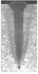
When the target is the evaluation of the exchanged energies, the results obtained from melting an indium sample (19.0 mg) using temperature programmed devices can show relevant differences depending on the sample positioning [12]. Figs. 2 show the change in the measured energy using a classical Differential Scanning Calorimeter 2910 MDSC, TA Instruments, 1997.
The energy depends on the radial position of the indium sample insi