THESIS
MANGROVE CLASSIFICATION ON ASTER VNIR
USING VEGETATION INDICES AND NEURAL NETWORK
STUDY CASE : BERAU DELTA - EAST KALIMANTAN
Hapsari Maharani
ID G051060041
This thesis submitted to
Graduate School of Bogor Agricultural University, Indonesia In fulfill of the requirement for the degree of
Master of Science in Information Technology for Natural Resource Management
GRADUATE SCHOOL
ACKNOWLEDGEMENTS
The author would like to express her deepest gratitude and affection to her supervisor Dr. Vincentius P. Siregar, DEA for his suggestion on the thesis and whose guidance proved extremely valuable in the completion of this study. The author also would like to acknowledge her special gratitude to her co-supervisor Dr. Antonius Bambang Wijanarto for his encouragement, valuable comment and suggestion in completing this research thesis.
The special appreciation to author’s family and friends for their continued support and encouragement throughout the period of study, making it successful and memorable.
Grateful appreciation is also conveyed to faculties, staff and friend at SEAMEO BIOTROP for helping author a lot to study in here. The author doesn’t want to forget thanks to her classmates who give the valuable help and kindness to him.
STATEMENT
I, Hapsari Maharani, hereby stated that this thesis entitled :
Mangrove Classification on ASTER VNIR using Vegetation Indices and Neural Network , Study Case : Berau Delta - East Kalimantan
Is the result of my own work during the period of June until September 2008 and that it has not been published before. The advisory committee and the external examiner have examined the content of this thesis.
Bogor, September 2008
Hapsari Maharani (2008). Mangrove Classification On Aster Vnir Using Vegetation Indices And Neural Network, Study Case : Berau Delta - East Kalimantan. Under the supervision of Vincentius P. Siregar and Antonius B. Wijanarto.
ABSTRACT
ASTER with its VNIR sensor have the capability for mapping vegetation. With the resolution of 15m x 15m, this image should be able to classify mangrove is more details than Landsat TM with resolution of 30m x 30m. Based on this, algorithms was applied to explore the capability of this image for classifying mangrove. These are Standard Back Propagation Neural Network and some vegetation indices (DVI, NDVI, SR, and the modified of these algorithm by using Natural Color Composite : NCC-DVI, NCC-NDVI, NCC-SR). While, as study area, Berau Delta, East Kalimantan is chosen because there are still may found many species of mangroves.
Each algorithm show different results, but almost all of them capable to classify mangrove into zone level, except modification of vegetation index algorithms. Standard Back Propagation Neural Network is not quite good for classifying mangrove, because it can generate pixels into lower number of classes. While, DVI, NDVI, and SR can classify mangrove into 4 class. Its rather low than Maximum Likelihood Supervised classification and ISODATA Unsupervised classification which produced 5 class. But, when modified vegetation index applied, it a different results. They can detect Nypa fruticans class clearly than other species. Even, by using NCC-NDVI and NCC-SR class Nypa still can differentiate into detailer condition.
The specific condition of the area of study where high frequency of rain, may cause the amount of water content in the vegetation become increase. Since gives influence in low value of NIR reflectance and high reflectance of RED channel, the modified algorithm of vegetation indices using NCC applied, and show result better than standard algorithm of vegetation indices.
Research Title Mangrove Classification on ASTER VNIR using Vegetation Indices and Neural Networks
Study Case : Berau Delta, East Kalimantan.
Name Hapsari Maharani Student ID G051060041
Study Program MSc in IT for Natural Resource Management
Approved by, Advisory Board
Dr.Ir. Vincentius P. Siregar,DEA Dr. Antonius B. Wijanarto Supervisor Co-Supervisor
Endorsed by,
Program Coordinator On Behalf of The Graduate School Master Program Secretary
Dr. Ir. Hartrisari Hardjomidjojo, DEA Dr. Ir. Naresworo Nugroho, MSi
TABLE OF CONTENTS
STATEMENT... i
ACKNOWLEDGEMENT ... ii
ABSTRACT... iii
APPROVAL SHEET ... iv
TABLE OF CONTENT ... v
LIST OF TABLE ... vi
LIST OF FIGURE... vii
I INTRODUCTION 1.1 Background ... 1
1.2 Objectives ... 2
II LITERATURE REVIEW 2.1 Mangrove vegetation ... 3
2.2 ASTER ... 4
2.2.1 Reflectance Characteristic of ASTER VNIR... 5
2.2.2 Mangrove Classification using ASTER... 8
2.3 Vegetation Indices ... 9
2.3.1 Simple Ratio Vegetation Index ... 10
2.3.2 Normalized Difference Vegetation Index ... 12
2.3.3 Difference Vegetation Index... 13
2.4 Natural Color Composite ... 13
2.5 Standard Back Propagation Neural Network (SBP) ... 14
2.6 Maximum Likelihood Supervised Classification... 17
III. METHODOLOGY 3.1 Area Description ... 18
3.2 Data and General Method ... 19
3.2.1 Data ... 19
3.2.2 General Method ... 23
ASTER Image Processing... 23
Water Masking... 24
Predicting Class of Mangrove by Histogram... 25
ISODATA Unsupervised and Labelling Class ... 26
Classification using Neural Network Supervised Classifier ... 27
Classification using Maximum Likelihood Supervised Classifier.... 28
Classification using Vegetation Indices Classifier ... 28
Result Analysis using Map and Histogram... 30
Data Validation ... 31
IV. RESULTS AND DISCUSSION 4.1 Synchronized ISODATA Unsupervised with Field Data ... 32
4.2.2 Validation... 40
4.3 Neural Network Classification... 42
4.3.1 Map and Histogram... 42
4.3.2 Validation... 45
4.4 Vegetation Indices ... 46
4.4.1 Difference Vegetation Index (DVI) ... 46
4.4.2 Normalized Difference Vegetation Index (NDVI) ... 48
4.4.3 Simple Ratio (SR) ... 50
4.4.4 NCC-DVI ... 52
4.4.5 NCC-NDVI ... 54
4.4.6 NCC-SR ... 57
V. CONCLUSIONS AND RECOMENDATIONS 5.1 Conclutions ... 60
5.2 Recomendations ... 62
LIST OF TABLE
Table 2.1 Principle application for each band of ASTER VNIR... 6
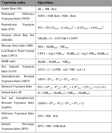
Table 2.2 Selected Remote Sensing Vegetation Index (Jensen 2000)... 11
Table 2.3 Parameters of ANN Classifier ... 17
Table 3.1 Scale Factor and Offset of ASTER VNIR Bands ... 24
Table 3.2 ASTER VNIR Natural Color Composite Algorithm and Real Channel... 29
LIST OF FIGURE
Figure 2.1 Zone of Mangrove from Beach to Land by Macnae (1966)... 4
Figure 2.2 ASTER Spectral Bands ... 5
Figure 2.3 Different reflectance signal of vegetation and dry soil (land) ... 6
Figure 2.4 Histograms of DN values in VNIR and SWIR... 9
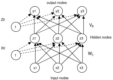
Figure 2.5 General Model of Standard Back Propagation neural Network ... 16
Figure 3.1 Landuse change in Berau Delta at last four years (2004 -2008) ... 18
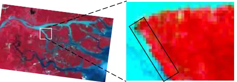
Figure 3.2. Research study area show in ASTER VNIR Berau Delta (2008) ... 20
Figure 3.3 Example of pixel checking by select area (about 1 km) that have specific condition and representative for training area ... 22
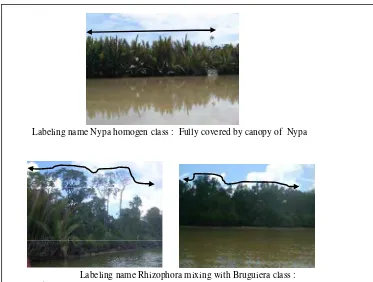
Figure 3.4. Example labeling class of mangrove based on dominant canopy coverage ... 22
Figure 3.5 General method steps ... 23
Figure 3.6 ASTER VNIR image masking water and cloud... 25
Figure 3.7 Histogram of each band represented class of mangrove vegetation.. 26
Figure 3.8 Model of Standard Back Propagation Neural Network... 28
Figure 3.9 ASTER VNIR with Natural Color Composite ... 30
Figure 4.1 ISODATA Unsupervised map and histogram of each class... 32
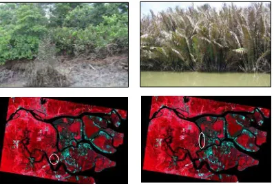
Figure 4.2 Result of field observation, Avicenia mixing with Nypa (left) and Rhizophora mixing with Nypa (right)... 35
Figure 4.3 Young Rhizopora mixing with young Nypa (left), and Nypa with un health condition (right) ... 35
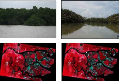
Figure 4.4. Rhizophora mixing with Bruguiera (left) and Nypa (right) ... 36
Figure 4.5 Condition of mangrove (burn and destroy) on Class 5... 37
Figure 4.6 Maximum Likelihood Supervised Classification map and histogram of each class ... 39
Figure 4.7 Map and Histogram of Neural Network classification... 42
Figure 4.8 Range of DN in Class 5, Class 2, and Class 4 on Band 1, Band 2, and Band 3N ... 44
Figure 4.9 Range of DN in Class 3 and 6 on Band 1, Band 2, and Band 3N ... 44
Figure 4.10 Map and Histogram derived from DVI Classifier ... 46
Figure 4.11 Map and Histogram derived from NDVI Classifier ... 48
Figure 4.12 Map and Histogram derived from SR Classifier ... 50
Figure 4.13 Map and Histogram derived from NCC-DVI Classifier ... 53
Figure 4.14 Map and Histogram derived from NCC-NDVI Classifier... 54
Figure 4.15 Sub Class 3A (left), 3B (middle), and 3C (right) ... 56
I.
INTRODUCTION
1.1 Background
It is well-known that the mangrove ecosystem plays important roles in coastal regions by its functions, which include supplying food and fuel wood for humans and natural protection against erosion. Moreover, mangrove ecosystem has become one of the key factors in considering the global warming issue and thus mangrove ecosystem is becoming increasingly important. However, mangrove mapping is quite a complex undertaking because of its distribution conditions, generally in high association.
Currently, various satellite data are available to assist mangrove area estimate throughout the world. They are Landsat TM, SPOT, ASTER, Quick Bird, ect,. In this research, ASTER with VNIR sensor chooses for studied the effectiveness in mapping and classification of mangrove. It is reported as an example of applying satellite data for mangrove management in Berau Delta, East Kalimantan.
Many method and approach used in vegetation classification, especially in mangrove. Generally, it is by selecting certain classification algorithm, like vegetation index algorithm. but it also other algorithms, such as k nearest neighbours, Expert System and Neural Networks (NN) (Walthall et.al., 2004).
THESIS
MANGROVE CLASSIFICATION ON ASTER VNIR
USING VEGETATION INDICES AND NEURAL NETWORK
STUDY CASE : BERAU DELTA - EAST KALIMANTAN
Hapsari Maharani
ID G051060041
This thesis submitted to
Graduate School of Bogor Agricultural University, Indonesia In fulfill of the requirement for the degree of
Master of Science in Information Technology for Natural Resource Management
GRADUATE SCHOOL
ACKNOWLEDGEMENTS
The author would like to express her deepest gratitude and affection to her supervisor Dr. Vincentius P. Siregar, DEA for his suggestion on the thesis and whose guidance proved extremely valuable in the completion of this study. The author also would like to acknowledge her special gratitude to her co-supervisor Dr. Antonius Bambang Wijanarto for his encouragement, valuable comment and suggestion in completing this research thesis.
The special appreciation to author’s family and friends for their continued support and encouragement throughout the period of study, making it successful and memorable.
Grateful appreciation is also conveyed to faculties, staff and friend at SEAMEO BIOTROP for helping author a lot to study in here. The author doesn’t want to forget thanks to her classmates who give the valuable help and kindness to him.
STATEMENT
I, Hapsari Maharani, hereby stated that this thesis entitled :
Mangrove Classification on ASTER VNIR using Vegetation Indices and Neural Network , Study Case : Berau Delta - East Kalimantan
Is the result of my own work during the period of June until September 2008 and that it has not been published before. The advisory committee and the external examiner have examined the content of this thesis.
Bogor, September 2008
Hapsari Maharani (2008). Mangrove Classification On Aster Vnir Using Vegetation Indices And Neural Network, Study Case : Berau Delta - East Kalimantan. Under the supervision of Vincentius P. Siregar and Antonius B. Wijanarto.
ABSTRACT
ASTER with its VNIR sensor have the capability for mapping vegetation. With the resolution of 15m x 15m, this image should be able to classify mangrove is more details than Landsat TM with resolution of 30m x 30m. Based on this, algorithms was applied to explore the capability of this image for classifying mangrove. These are Standard Back Propagation Neural Network and some vegetation indices (DVI, NDVI, SR, and the modified of these algorithm by using Natural Color Composite : NCC-DVI, NCC-NDVI, NCC-SR). While, as study area, Berau Delta, East Kalimantan is chosen because there are still may found many species of mangroves.
Each algorithm show different results, but almost all of them capable to classify mangrove into zone level, except modification of vegetation index algorithms. Standard Back Propagation Neural Network is not quite good for classifying mangrove, because it can generate pixels into lower number of classes. While, DVI, NDVI, and SR can classify mangrove into 4 class. Its rather low than Maximum Likelihood Supervised classification and ISODATA Unsupervised classification which produced 5 class. But, when modified vegetation index applied, it a different results. They can detect Nypa fruticans class clearly than other species. Even, by using NCC-NDVI and NCC-SR class Nypa still can differentiate into detailer condition.
The specific condition of the area of study where high frequency of rain, may cause the amount of water content in the vegetation become increase. Since gives influence in low value of NIR reflectance and high reflectance of RED channel, the modified algorithm of vegetation indices using NCC applied, and show result better than standard algorithm of vegetation indices.
Research Title Mangrove Classification on ASTER VNIR using Vegetation Indices and Neural Networks
Study Case : Berau Delta, East Kalimantan.
Name Hapsari Maharani Student ID G051060041
Study Program MSc in IT for Natural Resource Management
Approved by, Advisory Board
Dr.Ir. Vincentius P. Siregar,DEA Dr. Antonius B. Wijanarto Supervisor Co-Supervisor
Endorsed by,
Program Coordinator On Behalf of The Graduate School Master Program Secretary
Dr. Ir. Hartrisari Hardjomidjojo, DEA Dr. Ir. Naresworo Nugroho, MSi
TABLE OF CONTENTS
STATEMENT... i
ACKNOWLEDGEMENT ... ii
ABSTRACT... iii
APPROVAL SHEET ... iv
TABLE OF CONTENT ... v
LIST OF TABLE ... vi
LIST OF FIGURE... vii
I INTRODUCTION 1.1 Background ... 1
1.2 Objectives ... 2
II LITERATURE REVIEW 2.1 Mangrove vegetation ... 3
2.2 ASTER ... 4
2.2.1 Reflectance Characteristic of ASTER VNIR... 5
2.2.2 Mangrove Classification using ASTER... 8
2.3 Vegetation Indices ... 9
2.3.1 Simple Ratio Vegetation Index ... 10
2.3.2 Normalized Difference Vegetation Index ... 12
2.3.3 Difference Vegetation Index... 13
2.4 Natural Color Composite ... 13
2.5 Standard Back Propagation Neural Network (SBP) ... 14
2.6 Maximum Likelihood Supervised Classification... 17
III. METHODOLOGY 3.1 Area Description ... 18
3.2 Data and General Method ... 19
3.2.1 Data ... 19
3.2.2 General Method ... 23
ASTER Image Processing... 23
Water Masking... 24
Predicting Class of Mangrove by Histogram... 25
ISODATA Unsupervised and Labelling Class ... 26
Classification using Neural Network Supervised Classifier ... 27
Classification using Maximum Likelihood Supervised Classifier.... 28
Classification using Vegetation Indices Classifier ... 28
Result Analysis using Map and Histogram... 30
Data Validation ... 31
IV. RESULTS AND DISCUSSION 4.1 Synchronized ISODATA Unsupervised with Field Data ... 32
4.2.2 Validation... 40
4.3 Neural Network Classification... 42
4.3.1 Map and Histogram... 42
4.3.2 Validation... 45
4.4 Vegetation Indices ... 46
4.4.1 Difference Vegetation Index (DVI) ... 46
4.4.2 Normalized Difference Vegetation Index (NDVI) ... 48
4.4.3 Simple Ratio (SR) ... 50
4.4.4 NCC-DVI ... 52
4.4.5 NCC-NDVI ... 54
4.4.6 NCC-SR ... 57
V. CONCLUSIONS AND RECOMENDATIONS 5.1 Conclutions ... 60
5.2 Recomendations ... 62
LIST OF TABLE
Table 2.1 Principle application for each band of ASTER VNIR... 6
Table 2.2 Selected Remote Sensing Vegetation Index (Jensen 2000)... 11
Table 2.3 Parameters of ANN Classifier ... 17
Table 3.1 Scale Factor and Offset of ASTER VNIR Bands ... 24
Table 3.2 ASTER VNIR Natural Color Composite Algorithm and Real Channel... 29
LIST OF FIGURE
Figure 2.1 Zone of Mangrove from Beach to Land by Macnae (1966)... 4
Figure 2.2 ASTER Spectral Bands ... 5
Figure 2.3 Different reflectance signal of vegetation and dry soil (land) ... 6
Figure 2.4 Histograms of DN values in VNIR and SWIR... 9
Figure 2.5 General Model of Standard Back Propagation neural Network ... 16
Figure 3.1 Landuse change in Berau Delta at last four years (2004 -2008) ... 18
Figure 3.2. Research study area show in ASTER VNIR Berau Delta (2008) ... 20
Figure 3.3 Example of pixel checking by select area (about 1 km) that have specific condition and representative for training area ... 22
Figure 3.4. Example labeling class of mangrove based on dominant canopy coverage ... 22
Figure 3.5 General method steps ... 23
Figure 3.6 ASTER VNIR image masking water and cloud... 25
Figure 3.7 Histogram of each band represented class of mangrove vegetation.. 26
Figure 3.8 Model of Standard Back Propagation Neural Network... 28
Figure 3.9 ASTER VNIR with Natural Color Composite ... 30
Figure 4.1 ISODATA Unsupervised map and histogram of each class... 32
Figure 4.2 Result of field observation, Avicenia mixing with Nypa (left) and Rhizophora mixing with Nypa (right)... 35
Figure 4.3 Young Rhizopora mixing with young Nypa (left), and Nypa with un health condition (right) ... 35
Figure 4.4. Rhizophora mixing with Bruguiera (left) and Nypa (right) ... 36
Figure 4.5 Condition of mangrove (burn and destroy) on Class 5... 37
Figure 4.6 Maximum Likelihood Supervised Classification map and histogram of each class ... 39
Figure 4.7 Map and Histogram of Neural Network classification... 42
Figure 4.8 Range of DN in Class 5, Class 2, and Class 4 on Band 1, Band 2, and Band 3N ... 44
Figure 4.9 Range of DN in Class 3 and 6 on Band 1, Band 2, and Band 3N ... 44
Figure 4.10 Map and Histogram derived from DVI Classifier ... 46
Figure 4.11 Map and Histogram derived from NDVI Classifier ... 48
Figure 4.12 Map and Histogram derived from SR Classifier ... 50
Figure 4.13 Map and Histogram derived from NCC-DVI Classifier ... 53
Figure 4.14 Map and Histogram derived from NCC-NDVI Classifier... 54
Figure 4.15 Sub Class 3A (left), 3B (middle), and 3C (right) ... 56
I.
INTRODUCTION
1.1 Background
It is well-known that the mangrove ecosystem plays important roles in coastal regions by its functions, which include supplying food and fuel wood for humans and natural protection against erosion. Moreover, mangrove ecosystem has become one of the key factors in considering the global warming issue and thus mangrove ecosystem is becoming increasingly important. However, mangrove mapping is quite a complex undertaking because of its distribution conditions, generally in high association.
Currently, various satellite data are available to assist mangrove area estimate throughout the world. They are Landsat TM, SPOT, ASTER, Quick Bird, ect,. In this research, ASTER with VNIR sensor chooses for studied the effectiveness in mapping and classification of mangrove. It is reported as an example of applying satellite data for mangrove management in Berau Delta, East Kalimantan.
Many method and approach used in vegetation classification, especially in mangrove. Generally, it is by selecting certain classification algorithm, like vegetation index algorithm. but it also other algorithms, such as k nearest neighbours, Expert System and Neural Networks (NN) (Walthall et.al., 2004).
algorithm which also used are modification of each vegetation indices selected with Natural Color Composite. And the last are Maximum likelihood and Standard Back Propagation Neural Networks.
To find out which one the best algorithm for mangrove classification in estuary area become important, because it will help mapping mangrove indirectly (real ground mapping is almost impossible applied). Beside, hopely by using appropriate algorithm, it can reduce the bias effect of extraneous factors, such as soil and atmosphere easily.
1.2 Objectives
The main objectives of this research are :
1. To know the limitation of ASTER VNIR capabilities for mangrove classification, based on histogram of each bands.
2. To know capability of Standard Back Propagation Neural Network
for mangrove classification in ASTER VNIR.
3. To explore the selected vegetation indices algorithms (DVI, IPVI,
II. LITERATURE REVIEW
2.1 Mangrove vegetation
Mangrove describe as plant community that colonize the muddy shores of sheltered coast and river estuaries (Soepadmo, 1998). It dominant in tidal saline estuaries of tropical and subtropical (Twilley, 1998).
Being specific highly productive ecosystems and harbouring a large diversity of species adapted to these particular habitats, they are considered of almost ecological importance. Moreover, they provide a number of direct and indirect services, ranging from protection against coastal erosion (Pearce, 1999).
Santos et al (1997) mentioned that there are any factors that can influence mangrove distribution. Three main factors are beach physiographic, sea waves, and inundate periods. Beach physiographic will influence the composition, species distribution, and area of mangrove forest. On slightly beach, the variability of mangrove ecosystem is higher than steep beach. It is because there are wide place for mangrove growth. While, sea waves and inundate play as seed transportation.
subsided. Johnson and Frodin (1983) suggest one important factor, which also caused the zone of mangrove, that is bio-interaction.
Information about mangrove zonation will be helpful to predict the kind of mangrove species distribution, especially in the accuracy of mangrove mapping. Moreover, it also needs to make decision for coastal management.
Macnae (1966), devide zone of mangrove from beach to land as figure 2.1 follow :
a. Avicennia / Sonneratia zone b. Rhizopora zone
c. Rhizopora / Bruguiera zone d. Bruguiera zone
e. Nypa zone
2.2 ASTER (Advanced Spaceborne Thermal Emission and Reflection
Radiometer)
The ASTER instrument, provided by Japan's Ministry of International Trade and Industry and built by NEC, Mitsubishi Electronics Company and Fujitsu, Ltd., measures cloud properties, vegetation index, surface mineralogy, soil properties, surface temperature, and surface topography for selected regions of the Earth.
signal levels that are displayed as gray scale images from black to white, but they can obtain many images at the same time in different parts of the spectrum.
ASTER have three group of spectral bands. They are VNIR (Visible and NearInfrared), SWIR and TIR. Each of them have different resolution. VNIR is about 15 meter, SWIR is 30 meter, and TIR is 90 meter.
Figure 2.1 Zone of Mangrove from Beach to Land by Macnae (1966)
Figure 2.2 . ASTER Spectral Bands
2.2.1 Reflectance Characteristics of ASTER VNIR
Figure 2.3 Different Reflectance Signal of Vegetation and Dry Soil (Land)
ASTER VNIR have four band channel, green channel, red channel, NIR channel and NIR channel backward. The principles application for each bands is given in table 2.1. below.
Table 2.1 Principle Application for Each Band of ASTER VNIR
Band Wavelength Nominal Spectral
Location
Principle Application
1 520 – 600 nm Green Design to measure green reflectance peak of fegetation, vegetation discrimination and vigor assessment. Also usefull for cultural feature identification. 2 630 – 690 nm Red Designed to sense a chlorophyll
absorbtion region help in plant species differentiation. Also usefull for cultural feature identification
3N 760 – 860 nm Near Infrared Useful for determining vegetation types, vigor and biomass content, for delineating water bodies and soil moisture discrimination.
Reflectance signal of mangrove depend on pigment concentration and optical properties of leaves. Nevertheless, not all of satellite sensors easy to detect these factors. Need high resolution sensor capability to get exact result.
William and Norris (2001) reported that the limited number of spectral band of Landsat TM with resolution 30 meter, in which each band only covers a broad wavelength region of several tens of nanometers, offers a clear example of how opportunities to exploit spectral responses linked to the physico-chemical properties of plants are lost. Same cases with other satellite sensors, the broad spectral information of Landsat TM cannot be used to resolve several key absorption pits as well as reflectance characteristics including the red edge.
William and Norris (2001) added, the unique feature of plant spectral responses between the wavelength of 690 nm and 720 nm can be used to extract important physico-chemical characteristics of plants including chlorophyll contents. Base on this, the wavelength VNIR shown high information content for vegetation detection, because spectral of NIR 760 – 860 nm and VIS-red 630-690 nm.
2001). Spectral reflectance increases with wavelength and is a function of soil moisture (Stark et.al. 2000).
NIR reflectance is different in each species due to its independence on factors such as architecture of the canopy, cell structure and leaf inclination. Jackson and Pinter (1986) found that an erectophile canopy generally disperses more radiation in the lower layers than does a planophile canopy, consequently minimizing NIR reflectance. On other hand, reflectance in the visisble range is less specific on the species since it is mainly influenced by pigment content and composition (Gitelson et.al. 2002).
2.2.2 Mangrove Classification using ASTER
For classifying mangrove species, analysis of Band 1 to Band 9 spectra of ASTER was carry out for Can Gio Mangrove biosphere, in Vietnam. Mangrove’s digital number (DN) values in SWIR are generally lower than non-mangrove vegetation such as wild grass and rice paddy. Different mangrove species such as Avicennia alba, Rhizophora apiculata and Phoenix paludosa have different specific DN values. These spectral variations enable us to separate mangroves and classify mangrove species. In particular, different spectral pattern was observed in different mangroves (Hirose, 2006).
2.3 Vegetation Index
The identification of vegetation is of major interest, since leaves and needles constitute photosynthetic areas and a principal link between the biosphere and the atmosphere. Vegetation also has a distinctive spectral signature that is characterized by low reflectance in visible region of the solar optical spectrum as well as high reflectance in infrared spectrum. The combination of these two spectral regions can allow to classify vegetation and to determine the quantity of photosynthetic biomass by using vegetation density (Pinty and Verstraete, 1992).
Pinty and Verstraete (1992) added, that different combinations between visible and NIR bands have been used to develop various vegetation index based on image that the National Oceanic and Atmospheric Administration (NOAA) has obtained through its advanced very high resolution radiometer (AVHRR).
Vegetation index it self define as combination of several spectral values that are mathematically recombined to yield a single value indicating the amount or vigor of vegetation within pixel (Campbell, 1996). Most index have used reflectances from visible and infrared bands or radiances in the form of ratios or linear combinations.
Wavelength Digital number
A vegetation index was introduced as a simple remote sensing tool for over 25 years. Vegetation index have been used for many years of increasing importance in the field of remote sensing. Vegetation index was a number that is generated by some combination of remote sensing band and may have some relationship to the amount of vegetation in given image pixel. Remote sensing devices operated in the green, red, and NIR regions of the electromagnetic spectrum, they act as sensitive discriminators of variations in radiation output that measure both absorbtion and reflectance effects associated with vegetation.
There are more than 20 vegetation index in use are summarized in Table 2.1. many are functionally equivalent (redundant) in information content (Perry and Lautenschlager, 1984), while some provide unique biophysical information (Qi et.al. 1995). It is useful to review the historical development of the main indices and provide information about recent advances in index development.
2.4.1 Simple Ratio Vegetation Index (SR or RVI)
Cohen (1991) suggest that the first true vegetation index was the simple ratio (SR), which is the NIR to red reflectance ratio described in Birth and McVey (1968).
Table 2.2 Selected Remote Sensing Vegetation Index (Jensen 2000)
Vegetation index Algorithms
Simple Ratio (SR)
Normalized Difference
Vegetation Index (NDVI)
Perpendicular Vegetation
Index (PVI)
Greeness Above Bare Soil
(GRABS)
Moisture Stress Index (MSI)
Leaf Relative Water Content
Index (LWCI)
MidIR index
Soil Adjusted Vegetation
Index (SAVI)
Atmospherically Resistant
Vegetation Index (ARVI)
Enhanced Vegetation Index
Infrared Index (II)
Soil and Atmospherically
Resistant Vegetation Index
(SARVI)
Difference Vegetation Index
(DVI)
Infrared Percentage
Vegetation Index (IPVI)
SR = NIR / Red
NDVI = (NIR-Red) / (NIR + Red)
DVI = NIR – Red
IPVI = NIR / (NIR+Red)
II = (NIRtm4 – MidIRtm5) / (NIRtm4 + MidIRtm5)
SARVI = (P*nir – P*rb) / (P*nir + P*rb + L) ARVI = (P*nir – P*rb) / (P*nir + P*rb)
EVI = [(P*nir – P*red) / (P*nir + C1P*blue – C2P*blue + L)] (1+L) PVI =
√
(0.335mms4 - 0.149mms2)2 + (0.355mms2 – 0.852mms4)2GRABS = G – 0.09178B + 5.58959
MSI = MidIRTM5 / NIRTM4
LWCI = -log[1-(NIRtm4 – MidIRtm5)] / -log[1-NIRtm4-MidIRtm5]
MidIR = MidIRTM5 / NIRTM7
SAVI = (1 + L)(NIR - red) / NIR + red + L
2.4.2 Normalized Difference Vegetation Index (NDVI)
Rouse et.al., (1974) developed what is now called the generic Normalized Difference Vegetation Index (NDVI). NDVI is one of the ratio indices that respond to changes in amount of green biomass, chlorophyll content and canopy water stress. The healthy and dense vegetation show a large NDVI. Areas covered with clouds, water and snow, yield negative index value while areas covered with rock and bare soil result in vegetation indices near zero.
By comparing the visible and NIR light, scientist measure the relative amount of vegetation. Healthy and dense vegetation absorbs most of the visible light that hits it. Unhealthy and sparse vegetation reflects more visible light and less NIR. Mathematically NDVI is written as follow.
NDVI value range from minus one (-1.0) to plus one (+1.0) and are unitless (Wunderly et.al., 2003).
Environmental factors such as soil geomorphology and vegetation all influence NDVI values should be taken into account. NDVI can be effective in predicting surface properties when vegetation canopy is not too dense or too sparse. If a canopy too sparse, background signal e.g. soil can change NDVI significantly. Depending on the vegetation coverage, dark soil enhance the NDVI (Wunderly et.al., 2003). If the canopy too dense NDVI saturates because red reflectance does not change much, but NIR reflectance still increase when the canopy become denser.
2.4.3 Difference Vegetation Index (DVI)
Diference Vegetation index is a vegetation index obtained by subtracting the red reflectance from the NIR reflectance. The algorithm of DVI is show below.
DVI is proportional to NDVI. Here, DVI is simpler than NDVI but is prone to measurement errors in the NIR and red because it is not normalized by their sum. DVI also sensitive to the amount of the vegetation, and it has the ability to distinguish the soil and vegetation. But, DVI doesn’t give proper information when the reflected wavelengths are being effected due to topography, atmosphere and shadows.
2.4 Natural Color Composite on ASTER
Simulated natural color makes the imagery easy to understand by a wide range of users. Natural-color images are created from blue, green, and red light. Most satellite sensors do not collect data in the blue spectral band of the electromagnetic spectrum. Even when a blue band is available, the blue light, as seen from space, is scattered by atmospheric moisture (the reason for blue skies) creating a very noisy blue band, particularly in humid areas (Mather, 2004).
Terralook, USGS (2008) wrote that most satellite sensors collect near-infrared (NIR) data, which is sensitive to the health of vegetation. In response to the lack of a blue band and the availability of an information-rich NIR band, most satellite images are viewed using some combination of visible and infrared data.
ASTER images use the bands derived from the red, green, and NIR bands to derived the algorithm described below for a simulated natural-color image.
Red = Red
Green = 2/3 Green + 1/3 NIR Blue = 2/3 Green – 1/3 NIR
The synthetic green band is enhanced through the addition of information from the vegetation-sensitive NIR band. The synthetic blue is created from the spectrally-most-similar green band with the vegetation information suppressed.
2.5 Standard Back Propagation Neural Network (SBP)
There are different algorithm used to classify remote sensing images. The most often used of these, such as the maximum likelihood algorithm, require data with normal distribution. Among the algorithms that do not hypothesize on data distribution are the k nearest neighbours and neural networks (NN) (Walthall et.al., 2004).
correspond to input and output variables, respectively (Hilera and Martinez, 2000).
The Standard Back Propagation (SBP) architecture provided by PREDICT was used to perform classification. SBP is a method for training MLP (Multy Layer Percepton). This is a method for assigning responsibility for mismatches to each of the processing elements in the network, this is achieved by propagating the gradient of the objective function back through the network to the hidden units. Based on the degree of responsibility, the weight of each individual processing element are modify iteratively to improve the objective function. Input are supplied to the network and each input is given a weight, W. this weight is combined with other weights at the hidden layer node and a new weight is calculated. Weight modifications are made at all nodes then sent back between the first and second layers, until it reach the designed output error rate. An error rate is set to help evaluate the actual value against the predicted value. One node is assigned to each input data. Two parameters, momentum and leaning rates also affect the network.
When the pattern is presented to the input layer, it is evaluated by the hidden layer nodes, which pass on their output to the input layer. This can be thought of
as the forward phase. Next step is calculate δ(delta) on the output received from
this layer. The delta rule helps minimize the error on a gradient.
Each training of the output nodes using gradient descent which is basically getting error down the slope i.e. descending the gradient of the curve. This is the
hidden layer nodes. Hence the name is back propagation. The SBP is mathematically defined as :
∆Wij = ηδjοi
If unit j is an output unit, then δj = f’j (netj)(tj – Oj)
If unit j is a hidden unit, then δj = f’j (netj)
Σ
kδk WjkWhere :
η = learning parameter – specifies the step width of gradient descent
δj = tj – Oj = difference between teaching value tj and an output Oj of an
output unit which is propagated back.
f’j (netj) indicates function of which in this case would be define by the delta
[image:35.612.201.431.419.582.2]rule. This algorithm update the weights every training pattern.
Figure 2.5 General Model of Standard Back Propagation neural Network
A least squares objective function is minimized in a feed forward step followed by an error back propagation step during which the output and middle
Input nodes
Hidden nodes output nodes
Z0
X0
Wij
Vjk
1 1
x1 x2 x3
y1 y2 y3
layer weights are adjusted to reduce the size of error. This process is continued in an interactive fashion for each observation in the data set until some desired degree of error minimization or convergence is reached.
The following parameters were used with the PREDICT classifier :
Table 2.3 Parameters of ANN Classifier Hidden layer = 100 Learning rate
Output layer = 0.01
Learning rule Adaptive gradient Variable selection model Multiple regression Training and testing 10-fold cross validation
ANNs present a promising mode to improve classification of remotely sensed images. Many authors reported better accuracy when classifying spectral images with an ANN approach than with a statistical method such as maximum likelihood. However, a more important contribution of the ANNs is their ability to incorporate additional data into the classification process (Kaul et.al. 2005).
2.4 Maximum Likelihood Supervised Classification
III. METHODOLOGY
3.1 Area Description
Berau Delta, East Kalimantan is located between 1° 54’ 27’’ N – 2° 28’ 36’’N Lat and 117° 55’ 13’’E – 118° 26’ 12’’E Lon. Berau Delta is on estuary area which is composed by sediment material from Berau rivers and Maluku strait.
Berau Delta is one of the anthropogenic area of mangrove in Indonesia. It has similar condition with Mahakam delta about 10 years ago. But, during last four year, Berau delta have little changed. Some area was opened become ponds, and rural settlement. It is easy to detect with remote sensing data of ASTER VNIR 2004 (June 15th, 2004) compared with ASTER VNIR 2008 (June 22nd, 2008) on Figure 3.1
Field survey observation 2005, by BAKOSURTANAL reported that Berau river as small river, reaching 150 km inland, and the catchments basin has low anthropogenic pressure compared to other rivers of the region, so it has relatively low sediment delivery. This enables the presence of large diversity of marine and coastal habitat such as mangroves.
or crocodiles as a native fauna will decrease. In other side, the population of mangrove species it self also decrease because illegal loging.
ASTER VNIR 2004 ASTER VNIR 2008
Figure 3.1 Landuse Change in Berau Delta at Last Four Years (2004 -2008)
Based on the last field survey observation on middle of June 2008, the human activity in this delta is not too high. It can be indicated by the area of mangrove which is still higher than the thropogenic area. Although, the change of Berau Delta is still not significant, but it can indicate the sustainable of mangrove ecosystem on this area which is threatened.
3.2 Data and General Method 3.2.1 Data
a. Satellite Imagery Data
Figure 3.2. Research Study Area Show in ASTER VNIR Berau Delta (2008)
b. Field Data and Observation
The image has been checked on the field at middle of June 2008, the result show that the condition of mangrove have been changed, but it is not significant. Field data were taken by observation in rivers track from upland of delta until near the shore line. Transect methods cannot applied because the mangrove condition is very dense. Selection of location to be check is based on the domination of mangrove species. The reports of BAKOSURTANAL survey on 2005, 2006, and 2007, state that there are any specific condition of mangrove zonation in this delta. Nypa fruticans is dominated almost the half of the delta area. And the other are woods mangroves, such as Rhizopora sp. Bruguiera sp, and Avicenia sp. They are in the mixing and association condition, so its difficult to separate each other by visual interpretation.
Field observation have some objectives. It is for predicting the level of mangrove class, based on real condition of distribution each species. ASTER
VNIR 15m x 15m still may classify mangrove into level zone, not in species. It is based on two factors, pixel checking and labeling class of mangrove.
¾ Pixel checking
Pixel checking done by selecting area about 1 km which known have specific mangrove condition (As an example is Nypa area on Figure 3.3). Here, used 1 km area for avoid mistakes in position of pixel (pixel sliding when data of GPS tracking overlay into image). In 1 km area representative 67 pixels of ASTER. These group of pixels can used as training area selection in supervised classification, which representative one specific condition of mangrove class.
¾ Labeling Class of Mangrove
[image:41.612.202.446.570.655.2]The area where selected as training area have specific coverage canopy by certain mangrove species. This is usefully to know the dominant species of mangrove in the area, based on their reflectance. This way is very help in judge the class of mangrove when the condition is not homogen, such as Rhizopora sp mixing, Avicenia sp mixing, or Bruguiera sp mixing. The dominant canopy coverage by one or some species used to labeling the name of class. As an example is show in Figure 3.4.
Figure 3.4. Example Labeling Class of Mangrove Based on Dominant Canopy Coverage
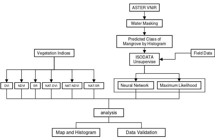
3.2.2 General Method
In general, the methods of this research can be seen in figure 3.5. ASTER with VNIR band has been separated from other 11 band of ASTER. Band 3B (backward) as part of visible band cannot be used, because it produce by different sensor of ASTER satellite. Band 3B looks backwards at an angle of 27.6 degree, so it not really vertically down. This band usually use to produce digital elevation model. Band composite that used in this research is False Color Composite 3N-2-1. While, the steps of each methods in this research explained below.
Labeling name Nypa homogen class : Fully covered by canopy of Nypa
Labeling name Rhizophora mixing with Bruguiera class :
Figure 3.5 General Method Steps
a. ASTER Image pre processing
Image processing is the first step in this research work. There are two main procedure, geometric correction and atmospheric correction. Geometric correction was done based on the vector to image registration. The vector data was used is hydrology map of Berau Delta, from BAKOSURTANAL. While, atmospheric correction done by dark pixels correction. Digital number (DN) of each band should be minus by minimum value of DN it self. Image with real digital number change into radiance unit, by adding with scale factor and multiply with offset. The equation is :
R = DN * scale factor + offset
Where R is reflectance value in radiance, DN is Digital Number of each band ASTER VNIR, and Scale factor and offset of each band show in table 3.1 below.
ASTER VNIR
Water Masking
Vegetation Indices
Predicted Class of Mangrove by Histogram
ISODATA Unsupervise
Field Data
Neural Network Maximum Likelihood
DVI NDVI SR NAT-DVI NAT-NDVI NAT-SR
analysis
Table 3.1 Scale Factor and Offset of ASTER VNIR Bands
b. Water Masking
Masking water and other object such as cloud and sediment by using formula editor to slicing the area only focus in land and vegetation. The aim is to reduce false in analysis, and therefore, the process of classification become easier. To mask water and other object, here using band 3N expressed NIR channel. Because assumption that NIR channel is more sensitive for object with high water content. Figure 3.6 show the result of image masking.
Figure 3.6 ASTER VNIR Image Masking Water and Cloud
Band Scale Factor Offset
1 0.676 - 0. 676
2 0.708 - 0.708
c. Predicting Class of Mangrove by Histogram
After the area of research mask in water and other object, histogram of ASTER VNIR bands compared each other to predict amount class of mangrove. This is shown in a number of peaks. The band, which has more peak than the other used as reference to derived number of mangrove class (the number of peak means number of mangrove class).While, the other band which have less number of peak will be neglected (Figure 3.7).
Based on the histogram of each bands, known that band 1 can derived into 12 class peaks, band 2 into 13 class peaks, and band 3N into 11 class peaks. This means that the number peaks of band 2 (Red channel) were used as reference for classifying mangrove.
Figure 3.7. Histogram of Each Band Represented Class of Mangrove Vegetation
Band 1 Band 2
d. ISODATA Unsupervised and Labeling Class by using Field Data
Unsupervised classification was done before each class has a name. The range of pixels value divide into 13 classes based on peaks of band 2. Afterwards, field data used for labeling the class was derived. It possibly, the number of class from field is quite different with the result from unsupervised classification. The factors that influence this condition will be analyzed and field data will be synchronized with the image classes.
e. Classification Using Neural Network Supervised Classifier
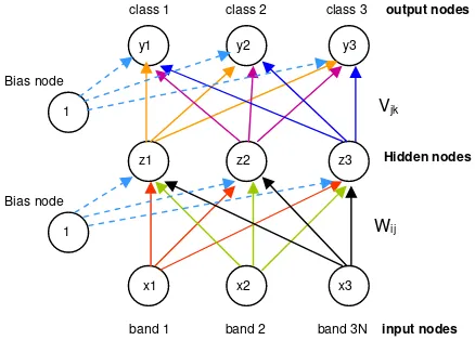
Before beginning the iteration, some parameters should be defined : input, output, and hidden layer. It also needs initialization process to standardized input into neural network value.
Input nodes are band 1, band 2, band 3N
Hidden layers = 1 learning rates
Output nodes are amount of class from unsupervised classification
Initialization :
Normalize input data band 1, band 2, band 3N value (0 -255) and target (tk) into range [0..1]. Then, gives random values between -1 to 1 for all Wij and Vjk
The iteration will start with feed forward step to predict target (tk). Target is not the real output value, but it calculate to get specific value for each class. Feed forward step it self devide into two step calculation. First, is calculate hidden nodes (Z1,Z2,Z3) and the second is calculate target output.
(0.3). The result of this calculation used to compute error of the nodes in input layer, and adjust weight Wij. (In this step also using constant value of learning rate
0.3).
[image:47.612.210.429.331.494.2]The iteration will stopped if output Y are close enough to target. The termination can be based on the error value. For instance, iteration process is stopped when error less than 0.0001 (this number is must be defined in ENVI 4.2 before iteration process). After being trained, the network can be used to predict certain classes by inputting value of each band. The general step show in figure 3.3.
Figure 3.3 Model of Standard Back Propagation Neural Network
f. Classification Using Maximum Likelihood Supervised Classifier
To produce mangrove map, supervised classification was used. A maximum likelihood supervised classification was carried out using training areas chosen according to the unsupervised classification which have been labeled. Afterwards,
band 1 band 2 band 3N input nodes
Hidden nodes
class 1 class 2 class 3 output nodes
Bias node
Bias node
Wij
Vjk
1 1
x1 x2 x3
y1 y2 y3
the raw result of the supervised classification was checked during visual interpretation of the satellite image and field data.
g. Classification using vegetation indices classifier
There are two type of vegetation indices applied in this research. First Standard vegetation index algorithms such as DVI, NDVI, and SR. While, second is algorithms using Natural Color Composites (NCC). Three standard vegetation indices have been selected from 14 vegetation indices algorithms. They are selected to derived map of mangrove because can be used in ASTER VNIR, and closely with NDVI, where generally used in many vegetation mapping and classification.
While, the modification algorithm using NCC applied by build synthetic layer green and blue on the image, before applied the vegetation indices algorithms (Figure 3.4). The equations of each layer become change (Table 3.2), also the algorithms of each standard vegetation index.
Table 3.2 ASTER VNIR Natural Color Composite algorithm and real channel
RGB Layer ASTER VNIR - NCC ASTER VNIR Channel
Red Red channel Red channel
Green (2/3*Green channel) + (1/3*NIR channel) Green channel
Blue (2/3*Green channel) - (1/3*NIR channel) NIR channel
a. NCC-DVI
The standard algorithm of DVI
NIR input change become blue layer of NCC
((2/3 * Green channel) - (1/3 * NIR channel)) - Red channel..…... (2)
b. NCC-NDVI
The standard algorithm of NDVI
NDVI = (NIR – RED / NIR + RED) ……… (1) NIR input change become blue layer of NCC
NCC-DVI / ((2/3*Green channel)-(1/3*NIR channel)+Red channel).. (2)
c. NCC-SR
The standard algorithm of SR
SR = NIR / RED …………..……… (1) NIR input change become blue layer of NCC
((2/3 * Green channel) - (1/3 * NIR channel))/ Red channel …... (2) Each algorithm of vegetation indices will applied into image. Its not based on unsupervised classification, but specific treatment.
h. Result Analysis Using Map and Histogram
The results of each classification methods in this research are shown in map and histogram. The focus of analysis are the number of mangrove classses that can be derived from each algorithm and the capability to mapping mangrove into certain level of class it self (zone, density, or species). One algorithms will not compared each other, but explored the capability for mangrove classification using ASTER VNIR data were explored.
i. Data Validation
IV. RESULT AND DISCUSSION
4.1 Synchronized ISODATA Unsupervised Classification with Field Data
The number of peak from ASTER VNIR bands express the capability of this
image to detect class of object on the field. Based on histogram of each band on Chapter
III, band 2 have more peaks than the other. It is quite different with the normal condition
of reflectance vegetation, because amount of water in the atmosphere and leaf is high.
When, observation was done on middle of June 2008 (the same date with ASTER image
captured) the frequency of rain at Berau delta is often, almost every day, even more than
a times in one day. So, leaf water content becomes increase. The reflectance of NIR was
low, while, Red was higher than normal. Because the NIR wavelength absorbed by water.
The impact, when ASTER VNIR image was analyzed, there were only few pixels
which have high value of Band 3, because not all of mangrove vegetation have same
capability to keep high amount of water in their leaf. The value of Band 3 will high, if the
mangrove leaf fast in past the water. In reality, the type of leaf and canopy gives high
influenced. Nypa with long leaf and almost vertically, will past the water faster than
Avicenia and Rhizophora. This means that the pixels which still have high value in Band
3 are pixels of class Nypa.
While, the condition of band 2 which more sensitive, it is easy to know because
the frequency of pixels are more various. This means that, these pixels not only express
class of Nypa, but also other kind of mangrove conditions. Based on this, band 2 was
classes of them are mangrove. The other 7 class are kind of land, and sediment. The last
one class is expressed pond.
Figure 4.1 ISODATA Unsupervised map and histogram of each class
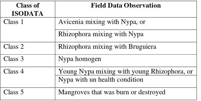
Field data as a result of observation and ground checking gives information in
certain area that is include into class of ISODATA unsupervised. When the information is
overlaid on the image, class 1 represents Avicenia mixing with Nypa or Rhizophora
mixing with Nypa, class 2 is Rhizophora mixing with Bruguiera, class 3 is Nypa
11.128 12.128
14.927
13.047
6.349
0 10 20 30 40 50
class 1 class 2 class 3 class 4 class 5 Kind of Class
P
e
rcen
ta
g
e
(
%
homogen, and class 4 is young Nypa mixing with young Rhizophora or Nypa with un
[image:53.612.137.482.181.354.2]health condition. These data show in Table 4.1 below.
Table 4.1 Synchronized Class of ISODATA and Field Data Observation
Class of
ISODATA
Field Data Observation
Avicenia mixing with Nypa, or
Class 1
Rhizophora mixing with Nypa
Class 2
Rhizophora mixing with Bruguiera
Class 3
Nypa homogen
Young Nypa mixing with young Rhizophora, or
Class 4
Nypa with un health condition
Class 5
Mangroves that was burn or destroyed
From ISODATA unsupervised classification, mangrove can split into five class,
while field observation have more than four class (7 class). This means that the capability
of ASTER VNIR for classifying mangrove is limited. As an example, Avicenia mixing
with Nypa or Rhizophora mixing with Nypa, still group into one class (Class 1). The
same condition with Class 4, where young Nypa mixing with young Rhizophora cannot
split with Nypa which un health condition.
It maybe other factors that influence the capability of ASTER VNIR for mapping
mangrove, there is a density of mangroves. In Class 1, Avicenia mixing with Nypa
cannot be separated from Rhizophora mixing with Nypa, because both classes almost
have the same density condition. On the map, yellow color on the near shoreline is class
class of Rhizophora mixing with Nypa. From field observation, both of them almost have
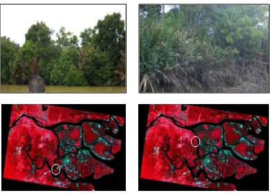
similar density. In figure 4.2, the photographs captured from the field, for both mixing
[image:54.612.88.480.192.472.2]conditions are shown.
Figure 4.2 Result of field observation, Avicenia mixing with Nypa (left) and Rhizophora
mixing with Nypa (right) and the corresponding ASTER image.
Class 4 cannot be seen on map clearly because the area is quite narrow. But, there
are two conditions based on field observation that can include into this class. The first is
condition of mixing young Rhizophora with young Nypa, and the second is un health
Nypa. Area growth by young Rhizophora and young Nypa are not really covered by their
canopy, it let the soil reflectance influenced the value of pixels. While, Nypa with un
(Figure 4.3). This means that the age of mangrove and healty condition become important
factor in mangrove classification. The young age and un health condition of mangrove
cause the reflectance higher and in reality they read as same object on the ASTER VNIR
image.
The widest area on the field also on the image is class 2. it is mixing between
Rhizophora and Bruguiera. While, Class 3, Nypa is the second widest area.
Figure 4.3 Young Rhizophora mixing with young Nypa (left), and Nypa with un health
condition (right) and the corresponding ASTER image.
Both kind of the area have similar character in their reflectance. Rhizophora mixing with
Bruguiera have very high density compared with the other mixing of mangrove, because
that they can reflecting light better, with low diffuse. Bruguiera and Rhizophora are kind
of woods mangrove, they have big stem and dense leaf when they adult. While, Nypa
have difference character of leaf and canopy. The area of canopy becomes wide because
the types of their leaf are almost vertical, but dense. So, the light that reflected by their
leaves almost the same with wide canopy of Rhizophora and Bruguiera. But, its is just
can judge in specific condition, where these vegetation have very high density. The
[image:56.612.94.490.308.579.2]result of field observation of both class show in Figure 4.4
Figure 4.4. Rhizophora mixing with Bruguiera (left) and Nypa (right) and the
corresponding ASTER image.
Class 5 with green color express condition of mangrove that was burned and
area is look like opened land. The reflectance value are quite different and cannot used to
identify certain class or species of mangroves. So, on the next discussion, this class will
not explained detail. The photograph which capture from the field, represent of Class 5
[image:57.612.161.441.207.478.2]show in Figure 4.5.
Figure 4.5 Condition of mangrove (burn and destroy) on Class 5, and the corresponding
ASTER image
Graph on Figure 4.1 as a result of ISODATA Classifier show that almost all of
classes split in same percentage. Class 1 about 11%, Class 2 about 12%, Class 3 about
14%, Class 4 about 13%, and Class 5 is about 6% more. The condition was caused by
the ISODATA classifier capability to devide the range of pixels value almost into the
This means that, by using ISODATA classifier, all class objects that want to
detect can be separated easily. But, it is possible that there are any other classes inside
class was define. The class object which easy to detect is Nypa on Class 3. On the
homogen condition like this, ISODATA Classifier still accurate to used. But, when the
condition of vegetation is not homogen, it really needs to be check on the field. While
Class 1 and Class 4 which have almost same percentage, in fact they cannot be defined as
one specific class of mangrove, because more specific, based on the field observation it
should be defined into two classes. So, that this is the reason supervised classification
4.2 Maximum Likelihood Supervised Classification
4.2.1 Map and Histogram
Maximum likelihood choose as one of the classifier in this research because it has
specific objective. Although it not include on the title of the thesis, but it need to test the
capability of Standard Back Propagation Neural Network Classifier, by comparing them
in capability to produced class. The result of this classifier reported that it can split
mangrove into six class, five class appropriate with ISODATA classifier, and one class
that detect as object non vegetation (class 6). Class 6 will not include into discussion,
because these objects are pond, sediment, and land.
The Figure 4.6 show that Class 4 is quite higher than the other (35% more). This
class represent young Nypa mixing with young Rhizophora or Nypa with un health
condition. Both condition cannot be separated by using maximum likelihood classifier
because the pixel value are almost the same. If it is forced to derive separate classes, the
accuracy become low and difficult to identify on the map.
In this research, maximum likelihood was capable to produce accurate map of
mangrove. It is because the basic of this method to make pattern in pixels reading is
absolutely depend on the training area. If the training area have good distribution in pixel
selection, the distance between the mean of each class will be narrow. Then, it can reach
the pixels which select to grouping into one class or certain class quite far from the mean.
Figure 4.6 Maximum Likelihood Supervised Classification map and histogram of each
class
The training area was chosen for class 4 have narrow distance mean. This means
that, they can reach pixel value are quite represent same reflectance, and cannot spit these
into difference class. This condition, can be used as a reason that the capability of
ASTER VNIR for mapping mangrove by using maximum likelihood methods limited on
level zone.
Class 1 also has same condition with class 4, where two kind of mangrove mixing
condition cannot split into difference class. The value of pixels only can group into one
class. While, for the homogeny condition like class of Nypa (class 3), and high density of
5.877 35.098 10.059 23.498 5.361 0 10 20 30 40 50
class 1 class 2 class 3 class 4 class 5
Kind of Class
Rhizophora mixing with Bruguiera (class 2) maximum likelihood more easy to split them
from other class.
The resulting classification using maximum likelihood might be expected to be
more accurate than the other supervised classifier, even than those produced by either the
parallelpiped or
k-
means classifier, it suggest by Mather (2004). Its because on this
classifier using training area that being used to provide estimates of the shapes of the
distribution of the membership of each class in the p-dimensional feature space as well as
the location of the center point of each class.
4.2.2
Validation
The confusion matrix is two dimensional matrix, where the row express reference,
and the column is interpretation result. The value in bold is true value of each class. If the
matrix is read, there are any different condition between interpretation result and
reference. This difference can analyze in each class.
If class 1 test, there are number of pixels on the map that include into class 2,
class 3, class 4, and also class 5 and class 6 on the reference. But, its not much, because
number of pixel which still read true as class 1 is higher than the other, its about 186731
pixels or more than 56% from total of pixels on class 1. the same condition with class 2,
class 3, class 4, class 5 and class 6. Although any pixels read as another class, but the true
pixels is quite high. All condition of pixels can produce overall accuracy, 95.512%.
Mather (2004), reported the good accuracy for classification is more than 75%, so this
class 1 class 2 class 3 class 4 class 5 class 6 Total
class 1 186731 4167 341 3611 7017 4262 206129
class 2 4237 835992 174 35147 11496 288 887334
class 3 302 152 379034 5125 47 2716 387376
class 4 3345 34753 5569 1283719 704 2733 1330823
class 5 7290 11216 49 806 206816 326 226503
class 6 4348 282 2594 2473 271 424626 434594
Total 206253 886562 387761 1330881 226351 434951 3472759
On class 2, many pixels of Rhizophora mixing with Bruguiera (886562) read as
young Nypa mixing with young Rhizophora or Nypa un health (class 4) on the reference.
In other side, on class 4, many pixels read as class 2 (35147). This condition can be
happen, because the selection of training area give the result that mean value of each
class is almost the same. So, the selection pixels to grouping in their class also have
resemble value. It may the pixels on class 2 where include into class 4 are pixels that
express Rhizophora and Bruguiera in young age or not too dense. While other class on
4.3 Neural Network Classification
4.3.1 Map and Histogram
Comparison of result map between Neural Network and Maximum likelihood
show that by using Neural Network the number class of mangrove become decreased.
There are many pixels generalized into other class.
Two class which cannot identify are Rhizophora mixing with Bruguiera and class
Nypa. The both of class have different reasons so they cannot differentiate on image.
The group of pixels which should be include in class Rhizophora mixing with Bruguiera,
detect as class Nypa un health and destroyed mangrove. While, pixels of Nypa homogen
include into class 6, where not analyze in this research (Class 6 is labeled as pond and
sediment).
The generalization of these pixels because of the capability of classifier is limited.
Neural network cannot identify the pattern of that’s class, as a consequence of vegetation
distribution pattern as continuous data.
Pattern in this case This means that the composition of digital number of each
band. On image classification this range build based on the algorithm of the classifier.
As an example, maximum likelihood able to differentiate class object based on normal
distribution. This classifier will grouping the pixels which still tolerant with the limitation
range that algorithm’s build. The same condition with Neural Network, the pattern of
digital number will build based on training area of each object. Training area of class 1
has certain value were derived from mean, the same condition with class 2, class 3, class
4, class 5 and class 6. This value called as expected output. The expected output it self
easy to differentiate object if composition of band 1, band 2, and band 3 of each object is
quite different (called as different pattern).
This means that even the selection of training area (manually) is quite good, but if
the pattern is not significant, neural network still cannot identify that’s pixels as unique
class. Here, vegetation is one kind of object that difficult to separately by neural network,
because the composition of band 1, band 2, and band 3 of each class is resemble.
The capability of neural network to generalized object vegetation, also support by
the weighting value and resolution of the image. Weighting value caused the limitation
between object become diffuse. So, in the last result the some different object will detect
as one object. While, the resolution of the image will influenced the resemble of
reflectance value. In this research, ASTER VNIR with resolution 15m x 15m, proved
cannot differentiate mangrove detail by using neural network classifier.
Class 2 as mixing of Rhizophora and Bruguiera, have certain pattern between
both class at the nearest of class 2, there are class 3 and class 4. Its simple to know on
Figure 4.8. Pattern of DN class 2 read as unknown pattern on intermediate two known
pattern. The main factor that influence the result of neural network classification is
weighting. B