...
Chaos-assisted capture of
irregular moons
Sergey A. Astakhov*, Andrew D. Burbanks†, Stephen Wiggins†
& David Farrelly*
*Department of Chemistry&Biochemistry, Utah State University, Logan, Utah 84322-0300, USA
†School of Mathematics, University of Bristol, Bristol BS8 1TW, UK
...
It has been thought1–3
that the capture of irregular moons—with non-circular orbits—by giant planets occurs by a process in which they are first temporarily trapped by gravity inside the planet’s Hill sphere (the region where planetary gravity
dom-inates over solar tides4). The capture of the moons is then made
permanent by dissipative energy loss (for example, gas drag3) or
planetary growth2. But the observed distributions of orbital
inclinations, which now include numerous newly discovered
moons5–8, cannot be explained using current models. Here we
show that irregular satellites are captured in a thin spatial region
where orbits are chaotic9, and that the resulting orbit is either
prograde or retrograde depending on the initial energy.
Dissipa-tion then switches these long-lived chaotic orbits10into nearby
regular (non-chaotic) zones from which escape is impossible. The chaotic layer therefore dictates the final inclinations of the captured moons. We confirm this with three-dimensional
Monte Carlo simulations that include nebular drag3,4,11, and
find good agreement with the observed inclination distributions
of irregular moons at Jupiter7and Saturn8. In particular, Saturn
has more prograde irregular moons than Jupiter, which we can explain as a result of the chaotic prograde progenitors being more efficiently swept away from Jupiter by its galilean moons.
The recent discoveries of large numbers of irregular satellites at Jupiter5–7and Saturn8are helping to shed new light on how planets capture other bodies1–3,12–22. It has been widely held, for example, that the observed preponderance of retrograde irregular moons at Jupiter is due mainly to the well known enhanced stability of retrograde orbits with large semimajor axis, a (refs 2, 20–22). However, Saturn’s family of irregulars is now known to contain a much more even mix of prograde and retrograde satellites than that of Jupiter5–8. Further, Saturn’s irregulars have similarly large semi-major axes (as compared to Jupiter’s moons) when expressed in planetary radii8. This rules out simple stability arguments as explanations for the markedly different distributions of moons observed at the two planets.
Here we study capture in the three-dimensional (3D) ‘spatial’ circular restricted three-body problem (CRTBP), taking the Sun– Jupiter–moon system as our primary example4. In a coordinate system rotating with the mean motion, but with the origin trans-formed to the planet, the spatial CRTBP hamiltonian4becomes:
H¼E
primaries;ais a collection of inessential constants; the total energy in the non-inertial frame,E, is related to the Jacobi constant through
CJ¼22E; andr¼ ðx;y;zÞandp¼ ðpx;py;pzÞare the coordinate
and momentum vectors of the test particle. Angular momentum, h¼ ðhx;hy;hzÞwherehz¼xpy2ypx;is now defined with respect to
the planet, as is most natural in a study of capture23.
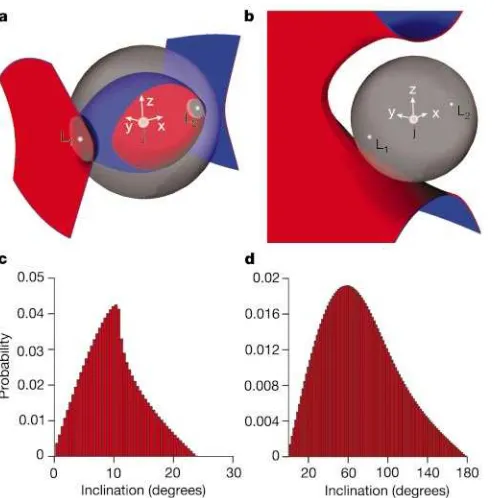
Figure 1a and b shows surfaces of zero velocity4at two energies for the 3D Sun–Jupiter system, together with the Hill sphere. Surfaces of zero velocity limit the motion in the rotating frame, and so serve to define an energetically accessible ‘bubble’ that may intersect the Hill sphere4. At both energies in Fig. 1, the two Lagrange saddle points, L1and L2, are ‘open’, and act as gateways between the interior
energy bubble and heliocentric orbits2,4. Figure 1c and d shows orbital inclination distributions4, i¼cos21ðh
z=jhjÞ; of test
par-ticles as they pass through the Hill sphere at the same two energies (see Methods). The key finding is that at energies slightly above the Lagrange points, only prograde orbits can enter (or leave) the capture zone. At higher capture energies, the distribution shifts to include both senses ofhz. The statistics of inclination distributions
will, therefore, be expected to depend strongly on energy, that is, the geometry of how (and if) the curves of zero velocity intersect the Hill sphere.
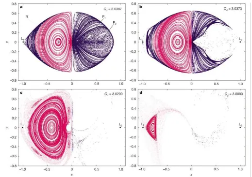
Figure 2 portrays the structure of phase space in the planar limit
ðz¼pz¼0Þin a series of Poincare´ surfaces of section9(SOS) at four
energies. At the lowest energy (Fig. 2a), many of the prograde orbits are chaotic, whereas all the retrograde orbits are regular9. Because incoming orbits cannot penetrate the regular Kolmogorov–Arnold– Moser (KAM) regions9, prograde orbits must remain prograde. Although KAM tori in 3D cannot ‘block’ trajectories in this manner, orbits can only enter nearly integrable volumes of phase space by Arnold diffusion, which, by the Nekhoroshev theorem, is expected to occur exponentially slowly9,10. In essence, the chaotic layer selects for the sense of the angular momentum of incoming and outgoing particles.
After L2has opened up (Fig. 2b), the chaotic ‘sea’ of prograde
orbits quickly ‘evaporates’, except for a thin, advancing front of chaos which clings to the KAM tori, buffering them from the expanding basin of direct scattering. With increasing energy, this
Figure 1The intersection of the Hill sphere in 3D with the surfaces of zero velocity, and histograms of inclination distributions for 108test particles originating at the Hill sphere.
Data are shown for two energies (aandc,bandd) for the Sun–Jupiter system with m¼9.5358£1024. In
aandcthe Jacobi constantCJ¼3.0380, and inbandd
CJ¼3.0100. The Lagrange saddle points are L1and L2. The coordinate system is
centred on Jupiter (small pink sphere, not to scale, labelled ‘j’). The Hill sphere is the large grey sphere.
letters to nature
NATURE | VOL 423 | 15 MAY 2003 | www.nature.com/nature
front smoothly shifts from prograde to retrograde motion. The surviving frontier tori are ‘sticky’, and chaotic orbits near them can become trapped in almost regular orbits for very long times10. Note that the KAM tori in Fig. 2 exist at energies above L1and L2, and so
dissipation need only be sufficient to switch chaotic orbits into the nearest KAM region for permanent capture to happen. At high energy, permanent capture is almost exclusively into retrograde KAM tori surrounding the almost circular, retrograde orbit, labelled R in Fig. 2a (refs 20, 21). The relative stability of prograde and retrograde orbits in two dimensions (2D) can be understood using Kapitza averaging (see Methods).
Figure 3 shows the normalized probability distribution of orbits from 3D Monte Carlo simulations which survive a cut-off time of 20,000 years; the distribution is shown as a function of the Jacobi constant and final inclination of the orbits. A clear trend from prograde to retrograde trapping with increasing total energy is found, which is consistent with Fig. 2. The three main structures visible in Fig. 3 correspond to low (prograde), intermediate and high (retrograde) inclinations. The large island ati<100–1208is related to librational motion around the argument of perijove q¼^908, that is, the Kozai resonance16,24. We confirmed numeri-cally that these distributions are similar for all the giant planets.
To understand further the role of chaos in shaping capture, we consider Hill’s approximation, which is valid (as here) form,,1; in appropriately scaled units, Hill’s equations contain no parameters, and so test-particle trajectories will scale accordingly for all the giant
planets4. This is confirmed by a comparison of SOS for the giant planets. Thus, the observed differences between Jupiter’s and Saturn’s families of irregulars probably cannot be explained using hamiltonian dynamics alone. However, significant differences may arise when a
Figure 2Poincare´ surfaces of section showing regions of chaotic (‘shotgun’ pattern) and regular (nested curves) dynamics. The surfaces are shown for randomly chosen initial conditions, and for the four indicated values ofCJ; units have been rescaled toRH¼1
(ref. 4). Points on the surface are coloured according to the sign of their angular
momentumhzas they penetrate thex–yplane; purple, prograde (hz.0); red,
retrograde (hz,0). Ina, P1, P2and R indicate two prograde and one retrograde periodic
orbit, respectively.
Figure 3The normalized probability distribution of 3D orbits that survived in Monte Carlo simulations (without dissipation) for 20,000 years. Data are shown as a function of their final inclination and initial value of the Jacobi constant. 80 million test particles were integrated, of which,38,000 survived for 5,000 years and,23,000 survived for
20,000 years. Using time-averaged inclinations with moving windows of 100–1,000 years produces essentially identical distributions. In these simulations, test particles were removed if they came within two planetary radii of the planet.
letters to nature
particle’s motion is dependent on additional perturbations that do not follow Hill’s scaling (for example, nebular gas-drag4,11).
In addition, the local environment at each planet is different; one such variable is the volume of the Hill sphere occupied by the massive, regular moons. This observation is important, because prograde orbits penetrate much deeper towards the planet than do most of the retrograde orbits (Fig. 2b and d). Therefore, to be permanently captured, prograde orbits (especially) must survive close encounters or collisions with the massive regular moons. Orbits in the chaotic layer may be very long lived, and so can cross the orbits of the inner satellites many times; and because chaotic orbits are rather sensitive to perturbations9, such passages will strongly perturb their orbital elements. Therefore, in our simulations with dissipation, we eliminated test particles that crossed the outermost massive regular moons of Jupiter and Saturn. We decided to use Saturn’s moon Titan (which is similar in mass to Jupiter’s outermost moon Callisto), rather than Saturn’s actual outermost, but significantly smaller, regular moon Iapetus4.
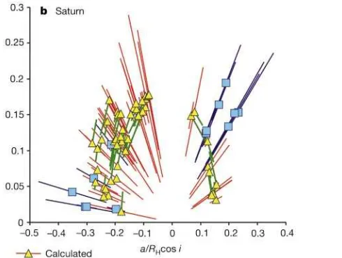
The results of these simulations (see Methods) are shown in Fig. 4. Saturn has a clear tendency to capture a higher ratio of prograde to retrograde moons as compared to Jupiter. This can be traced to the fact that Callisto’s semimajor axis is a larger fraction of the Hill radius for Jupiter (3.55%) than is the case for Titan, whose orbit is only 1.84% of Saturn’s Hill radius. This effect was confirmed in the simulations by moving Titan’s orbit out to the same relative distance (as a fraction of the Hill radius) as Callisto, which resulted in a prograde-poor distribution at Saturn, similar to that at Jupiter. Thus, the relative scarcity of jovian prograde irregulars may be due to their chaotic prograde progenitors having been swept away more efficiently by Jupiter’s galilean moons.
The inclinations of captured test particles (Fig. 4) compare well with observed inclinations, and similarly seem to occur in definite clusters and sub-clusters. All of these clusters originated in initially chaotic orbits, which originated on the Hill sphere. Remarkably, these orbits nevertheless tend to preserve their initial inclinations. This phenomenon of ‘inclination memory’ suggests that the observed clusters of irregular moons might be relics of the capture dynamics, rather than being necessarily the result of post-capture fragmentation through collisions3,8,12. For example, whereas average satellite inclinations are clustered, other orbital elements such as average eccentricity may be more widely dispersed; this is more
difficult to explain in a collision model5–8. A test of the fragmenta-tion hypothesis will come from more detailed observafragmenta-tions of the physical characteristics of irregular moons. These observations will also be a test of our model, which provides a single, unified, mechanism for the capture of both prograde and retrograde moons2,15,20–22.
Chaos-assisted capture may be involved in the formation of asteroid or Kuiper-belt binaries25, and also has implications for the feasibility of the capture of massive bodies such as Neptune’s retrograde moon Triton26. Figure 3 indicates that a moon captured into a high-inclination orbit would probably have first been trapped in the chaotic layer close to an almost-circular orbit (labelled R in Fig. 2); this provides a possible clue to the origin of Triton’s circular,
highly inclined orbit26. A
Methods
Monte Carlo simulations
An isotropic flux of test particles was originated in 3D on the Hill sphere (radiusRH¼
apðm=3Þ1=3whereapis the planet’s semimajor axis), and integrated until one of the
following occurred: the particle left the Hill sphere; it penetrated a sphere, centred on the planet, of a given radius (see figure captions and text); or it survived for a predetermined
cut-off time. Initial conditions were generated as follows: the vectorrwas chosen
uniformly and randomly on the surface of the Hill sphere. Velocities were also chosen uniformly and randomly in accordance with the value of the Jacobi constant. This
constant was chosen randomly and uniformly:CJ[ð2:995;CðJ1ÞÞ;whereC
ð1Þ
J is the value of
CJat L1. Figure 1c and d show the resulting distributions of initial inclinations for these
initial conditions. Numerical integrations were done using a Bulirsch–Stoer procedure27.
Choosing particles on the Hill sphere, where the motion is chaotic or scattering22,
minimizes the risk of accidentally starting orbits deep inside impenetrable KAM regions18.
Although permanently bound, such orbits could never in fact have been trapped, because KAM regions cannot be penetrated in 2D and only exponentially slowly in 3D. It is only in the thin chaotic layer between scattering and stability that capture can happen. This method of selecting initial conditions thus specifically selects for these particles.
Surfaces of section
The SOS9were computed by integrating randomly chosen ensembles of test particles with
initial conditions chosen inside the Hill radius (RH) and integrated using Levi–Civita
regularizing coordinates28. The SOS chosen is thex–yplane withp
x¼0 andy˙.0; points
have been coloured in Fig. 2 according to the sign of their angular momentum as they
intersect that surface. In almost all cases the sign ofhzis well conserved.
Simulations with dissipation
We integrated trajectories including a dissipative force representing nebular drag4,F
drag¼
2gv¼2gð_x;y_;_zÞ;wheregis the drag parameter. This form was chosen not only for its
simplicity, but also because it scales in the Hill approximation, which allowed for a more even-handed comparison of Jupiter and Saturn. This is true even in the CRTBP, for which
Figure 4Comparison of the orbital properties of the known irregular satellites of Jupiter5,6 (to 20027) and Saturn8with dissipative Monte Carlo simulations. The radial distance from the origin represents the moon’s orbital semimajor axis,a, as a fraction ofRH. The length
of each line shows the pericentre-to-apocentre distance of the orbit. Time-averaged
orbital elements are used. The green lines show the total excursion in inclination undergone by each moon. In most cases, a strong correlation between initial and final inclination is observed. In some cases, initial and final inclinations are indistinguishable on this scale.
letters to nature
NATURE | VOL 423 | 15 MAY 2003 | www.nature.com/nature
Hill’s scaling is only approximate. Experimental simulations revealed that, for fixed
integration times, the main effect of changinggwas to influence the final average values of
the semimajor axes of captured moons with respect to the planet; in contrast, the final inclination distributions were quite robust to the precise value of this parameter. Thus we
chosegheuristically so that the captured moons ended up roughly in the observed
semimajor axis ranges; we setg¼7£1025in units scaled for Jupiter, andg¼2
£1024 in units scaled for Saturn.
Integrations were performed for both Jupiter and Saturn for a maximum of 10,000 years for each test particle. Integrations were stopped, as explained in the text, if test particles crossed the orbit of Callisto (at Jupiter) or Titan (at Saturn), or if they left the Hill sphere. The simulations reported in Fig. 4 were stopped when 50 moons had been captured, but computations in which several thousand moons were captured produce similar results. We have also performed parallel simulations in the elliptic restricted three-body problem for Jupiter and Saturn, and also used different forms of dissipation—for example, nebular
gas-drag,Fdrag¼2gjvjv(ref. 11). All of these variations produced comparable results.
Kapitza averaging
The relative stability of prograde and retrograde orbits in 2D can be understood qualitatively by Taylor expansion of the solar part of the CRTBP hamiltonian, followed by
Kapitza averaging in plane polar coordinates over the angleJconjugate tohz. This is
similar to the analogous problem of ionization (escape) of an electron from a hydrogen
atom in a rotating field29,30. As in the atomic problem, this strategy produces an effective
potential whose saddle point is higher for one sense of angular momentum: in this case, the retrograde orbits, which are therefore more stable than the prograde orbits. Further,
using methods similar to those in ref. 23, it is possible to show thathzis the lowest-order
term in an approximate ‘third-integral’ valid inside the Hill sphere.
Received 6 December 2002; accepted 26 March 2003; doi:10.1038/nature01622.
1. Peale, S. J. Origin and evolution of the natural satellites.Annu. Rev. Astron. Astrophys.37,533–602 (1999).
2. Heppenheimer, T. A. & Porco, C. New contributions to the problem of capture.Icarus30,385–401 (1977).
3. Pollack, J. R., Burns, J. A. & Tauber, M. E. Gas drag in primordial circumplanetary envelopes: A mechanism for satellite capture.Icarus37,587–611 (1979).
4. Murray, C. D. & Dermot, S. F.Solar System Dynamics(Cambridge Univ. Press, Cambridge, 1999). 5. Shephard, S. S., Jewitt, D. C., Fernandez, Y. R., Magnier, G. & Marsden, B. G. Satellites of Jupiter.IAU
Circ. No., 7555 (2001).
6. Shephard, S. S., Jewitt, D. C., Kleyna, J., Marsden, B. G. & Jacobson, R. Satellites of Jupiter.IAU Circ. No., 7900 (2002).
7. Shephard, S. S.et al.Satellites of Jupiter.IAU Circ. No., 8087 (2003).
8. Gladman, B. J.et al.Discovery of 12 satellites of Saturn exhibiting orbital clustering.Nature412, 163–166 (2001).
9. Lichtenberg, A. J. & Lieberman, M. A.Regular and Chaotic Dynamics, 2nd edn 174–183 (Springer, New York, 1992).
10. Perry, A. D. & Wiggins, S. KAM tori are very sticky: rigorous lower bounds on the time to move from an invariant Lagrangian torus with linear flow.Physica D71,102–121 (1994).
11. Kary, D. M., Lissauer, J. J. & Greenzweig, Y. Nebular gas drag and planetary accretion.Icarus106, 288–307 (1993).
12. Colombo, G. & Franklin, F. A. On the formation of the outer satellite group of Jupiter.Icarus15, 186–189 (1971).
13. Huang, T.-Y. & Innanen, K. A. The gravitational escape/capture of planetary satellites.Astron. J.88, 1537–1547 (1983).
14. Murison, M. A. The fractal dynamics of satellite capture in the circular restricted three-body problem. Astron. J.98,2346–2359 (1989).
15. Namouni, F. Secular interactions of coorbiting objects.Icarus137,293–314 (1999).
16. Carruba, V., Burns, J. A., Nicholson, P. D. & Gladman, B. J. On the inclination distribution of the Jovian irregular satellites.Icarus158,434–449 (2002).
17. Nesvorn’y, D., Thomas, F., Ferraz-Mello, S. & Morbidelli, A. A perturbative treatment of co-orbital motion.Celest. Mech. Dynam. Astron.82,323–361 (2002).
18. Vieira Neto, E. & Winter, O. C. Time analysis for temporary gravitational capture: satellites of Uranus. Astron. J122,440–448 (2001).
19. Marzani, F. & Scholl, H. Capture of Trojans by a growing proto-Jupiter.Icarus131,41–51 (1998). 20. Henon, M. Numerical exploration of the restricted problem. VI. Hill’s case: non-periodic orbits.
Astron. Astrophys.9,24–36 (1970).
21. Winter, O. C. & Vieira Neto, E. Time analysis for temporary gravitational capture: stable orbits. Astron. Astrophys.377,1119–1127 (2001).
22. Saha, P. & Tremaine, S. The orbits of the retrograde Jovian satellites.Icarus106,549–562 (1993). 23. Contopolous, G. The “third” integral in the restricted three-body problem.Astrophys. J.142,802–804
(1965).
24. Kozai, Y. Secular perturbations of asteroids with high inclinations and eccentricities.Astron. J.67, 591–598 (1962).
25. Goldreich, P., Lithwick, Y. & Sari, R. Formation of Kuiper-belt binaries by dynamical friction and three-body encounters.Nature420,643–646 (2002).
26. Stern, S. A. & McKinnon, W. B. Triton’s surface age and impactor population revisited in light of Kuiper Belt fluxes: Evidence for small Kuiper Belt objects and recent geological activity.Astron. J.119, 945–952 (2000).
27. Press, W. H., Teukolsky, S. A., Vetterling, W. T. & Flannery, B. P.Numerical Recipes in C, 2nd edn 724–732 (Cambridge Univ. Press, Cambridge, 1999).
28. Aarseth, S. From NBODY1 to NBODY6: The growth of an industry.Publ. Astron. Soc. Pacif.111, 1333–1346 (1999).
29. Brunello, A. F., Uzer, T. & Farrelly, D. Hydrogen atom in circularly polarized microwaves: Chaotic ionization via core scattering.Phys. Rev. A55,3730–3745 (1997).
30. Lee, E., Brunello, A. F. & Farrelly, D. Coherent states in a Rydberg atom: Classical dynamics.Phys. Rev. A55,2203–2221 (1997).
AcknowledgementsThis work was supported by the US National Science Foundation, the Royal Society (UK) and the US Office of Naval Research.
Competing interests statementThe authors declare that they have no competing financial interests.
Correspondenceand requests for materials should be addressed to S.W. ([email protected]) or D.F. ([email protected]).
...
A theory of power-law distributions
in financial market fluctuations
Xavier Gabaix*, Parameswaran Gopikrishnan†‡, Vasiliki Plerou†
& H. Eugene Stanley†
*Department of Economics, Massachusetts Institute of Technology, Cambridge, Massachusetts 02142, USA
†Center for Polymer Studies and Department of Physics, Boston University, Boston, Massachusetts 02215, USA
... Insights into the dynamics of a complex system are often gained by focusing on large fluctuations. For the financial system, huge databases now exist that facilitate the analysis of large
fluctua-tions and the characterization of their statistical behaviour1,2.
Power laws appear to describe histograms of relevant financial fluctuations, such as fluctuations in stock price, trading volume
and the number of trades3–10. Surprisingly, the exponents that
characterize these power laws are similar for different types and sizes of markets, for different market trends and even for different countries—suggesting that a generic theoretical basis may underlie these phenomena. Here we propose a model, based on a plausible set of assumptions, which provides an explanation for these empirical power laws. Our model is based on the hypothesis that large movements in stock market activity arise from the trades of large participants. Starting from an empirical characterization of the size distribution of those large market participants (mutual funds), we show that the power laws observed in financial data arise when the trading behaviour is performed in an optimal way. Our model additionally explains certain striking empirical regularities that describe the relation-ship between large fluctuations in prices, trading volume and the number of trades.
Defineptas the price of a given stock and the stock price ‘return’ rt as the change of the logarithm of stock price in a given time
intervalDt;rt;lnpt2lnpt2Dt:The probability that a return has an
absolute value larger thanxis found empirically to be (see Fig. 1)4,8:
Pðjrtj.xÞ,x2zr ð1Þ withzr<3. Empirical studies also show that the distribution of trading volumeVtobeys a similar power law9:
PðVt.xÞ,x2zV ð2Þ withzV<1:5;while the number of tradesNtobeys10:
PðNt.xÞ,x2zN ð3Þ withzN<3.4.
The ‘inverse cubic law’ of equation (1) is rather ‘universal’, holding over as many as 80 standard deviations for some stock markets, withDtranging from one minute to one month, across different sizes of stocks, different time periods, and also for different stock market indices4,8. Moreover, the most extreme events—includ-ing the 1929 and 1987 market crashes—conform to equation (1),
‡ Present address: Goldman Sachs and Co., 10 Hanover Square, New York, New York 10005, USA.
letters to nature
NATURE | VOL 423 | 15 MAY 2003 | www.nature.com/nature ©2003 Nature Publishing Group 267