ISSN: 1693-6930
accredited by DGHE (DIKTI), Decree No: 51/Dikti/Kep/2010 531
Optic Nerve Head Segmentation Using Hough
Transform and Active Contours
Handayani Tjandrasa*, Ari Wijayanti, Nanik Suciati Sepuluh Nopember Institute of Technology (ITS)
ITS Campus, Sukolilo, Surabaya, Indonesia Telp/fax.: +6231-5939214/+6231-5913804
e-mail: [email protected]*
Abstrak
Optic nerve head merupakan bagian retina tempat sel ganglion axon keluar dari mata untuk membentuk optic nerve. Hilangnya fiber saraf akibat glaucoma menurunkan ukuran optic disk dan melebarkan ukuran cup. Karenanya evaluasi optic nerve head adalah penting untuk diagnosis dini glaucoma. Studi ini mengimplementasikan deteksi optic nerve head pada citra fundus retina berdasarkan Hough Transform dan Active Contour Model. Proses dimulai dengan perbaikan citra menggunakan filter homomorphic untuk koreksi iluminasi, kemudian dilanjutkan dengan penghapusan pembuluh darah untuk memfasilitasi proses segmentasi berikutnya. Hasil lingkaran transformasi Hough menjadi level set awal untuk active contour model. Hasil uji coba menunjukkan bahwa algoritma segmentasi mampu mendeteksi optic nerve head dengan akurasi rata-rata sebesar 75.56% dengan menggunakan 30 citra retina dari DRIVE database.
Kata kunci: active contours, citra fundus retina, optic nerve head, transformasi Hough
Abstract
Optic nerve head is part of the retina where ganglion cell axons exit the eye to form the optic nerve. Glaucomatous changes related to loss of the nerve fibers decrease the neuroretinal rim and expand the area and volume of the cup. Therefore optic nerve head evaluation is important for early diagnosis of glaucoma. This study implements the detection of the optic nerve head in retinal fundus images based on the Hough Transform and Active Contour Models. The process starts with the image enhancement using homomorphic filtering for illumination correction, then proceeds with the removal of blood vessels on the image to facilitate the subsequent segmentation process. The result of the Hough Transform fitting circle becomes the initial level set for the active contour model. The experimental results show that the implemented segmentation algorithms are capable of segmenting optic nerve head with the average accuracy of 75.56% using 30 retinal images from the DRIVE database.
Keywords: active contours, Hough transform, optic nerve head, retinal fundus image
1. Introduction
Glaucoma is the second most common cause of blindness on worldwide. In developed countries, less than 50% persons with glaucoma are aware of their disease [1]. Early diagnosis of glaucoma is important as early treatment can reduce the rate of blindness 20 years later by about 50% [2].Glaucoma is characterized by a progressive damage to the optic nerve. If it is not diagnosed and treated, it can lead to vision loss and blindness. Damage of the optic nerve is usually associated with the elevated eye pressure. Glaucomatous changes related to the loss of the nerve fibers decrease the neuroretinal rim and expand the area and volume of the cup. The measurement of optic disk morphological parameters is important for early diagnosis of glaucoma since the morphological changes precede visual field defects. Disk size evaluation is an important part of optic disk assessment to diagnose glaucoma, in addition to features such as neuroretinal rim and cup area. But it should be considered that the patient characteristics and the measurement method may affect the disk size estimates [3].
extraction, and classification. Segmentation of the optic disk was also developed using a morphological approach [6]. Patton et al. [7] outlined various methods for retinal digital image analysis. The work of Winder et al. [8] examined literature on digital image processing in the field of diabetic retinopathy to provide guidance to algorithm designers for diabetic retinopathy. Niemeijer et al.[9] developed fast method to detect the fovea and the optic disc by making few assumptions about the location. Welfer et al. employed detection of the optic disk location to identify the optic disk boundary using the Watershed Transform [10].
This study develops a system to detect the optic disk in retinal fundus images which consists of image enhancement and vessel removal filtering for segmentation preprocessing; Hough transform and Active Contour Models for optic disk segmentation. In our system, each step can be readily followed and implemented, such the developed software can be utilized for detecting other retinal features such as fovea and macula to give an integrated system for detecting other retinopathologies including diabetic retinopahy, hypertension, and age-related macular degeneration.
2. Research Method
The optic disk segmentation is preceded by converting a color retinal fundus image into a grayscale image, enhancing the image, and removing its blood vessels and the objects which are darker than its background and the optic disk. The segmentation process is divided in two stages. The first stage is a coarse segmentation of optic nerve head. In this stage, the location of the circle optic nerve head is detected using Hough transform. The next stage is to conduct the process of active contour model to obtain the form of optic nerve head that comes closer to its original form. The diagram for preprocessing and segmentation process is shown in Figure1.
Input optic disk
Image contour
Figure 1. Diagram of the segmentation process
2.1. Image Enhancement
The earliest stage in this implementation is image preprocessing. This process is done to compensate the effects of non-uniform illumination on an image. The image used is a color retinal fundus image of DRIVE database [11] that has been cropped to size 185 x 172 pixels. Homomorphic filtering method is used to suppress the effects of uneven illumination while keeping the intensity discrepancies among all the components in the image. Homomorphic filtering method has the following stages [12]:
a. Apply a Gaussian low-pass filter G(u,v) on the Fourier domain of the logarithmic of I(x,y), i.e. I(u,v), to get the filtered image I’(u,v).
I(u,v) = F(ln(I(x,y))) = F(ln(i(x,y))) + F(ln(r(x,y))) (1)
I’(u,v) = G(u,v) . I(u,v) (2)
ܩሺݑ,ݒሻ=
√݁
(మ మ)/మ
(3)
Invert-transform I' into spatial domain and take antilogarithm to obtain a filtered homomorphic image.
I’(x,y) = ln -1F -1(I’(u,v)) (4)
b. Perform dilation D to get back the filtered edge. Remove the effect of illumination from the original image by dividing it with dilated homomorphic view of the illumination of the original
Image
enhancement Vessel removal
image. This process produces a homomorphic filtered image I*, which appears to have uniformly distributed illumination.
ܫ∗ሺݔ,ݕሻ= (,)
(′(,))= ݅∗ሺݔ,ݕሻ.ݎ∗(ݔ,ݕ) (5)
݅∗(ݔ,ݕ) and ݎ∗(ݔ,ݕ) represent illumination and reflectance correspondingly.
The result of this process is a grayscale image with uniform illumination effect which facilitates the next process for the removal of blood vessels and nerve fibers in the image.
2.2. Blood Vessel Removal Process
After the preprocessing step that produces an image with uniform illumination, the next step is to remove the blood vessels and nerve fibers in the image, because these objects are not required in the segmentation process. Blood vessels and nerve fibers are detected from the low pixel values in the image by thresholding. The threshold is selected as 50 plus the minimum integer value of the image gray level. Next, the median filter of the size 41 x 41 is applied on the detected pixels to blur the blood vessels and nerve fibers.
2.3. Hough Transform for Circle Detection
Circle Hough transform can be described as transformation from every point on a circle in the xy space [13], [14]:
ܴ= (ݔ−ܽ)+ (ݕ−ܾ) (6)
Or in the parametric equations:
ݔ=ܽ+ܴܿݏ(ߠ)
ݕ=ܾ+ܴݏ݅݊(ߠ) (7)
Into the parameter space:
a = x1 – Rcosθ
b = y1 – Rsinθ (8)
for a particular point (x1, y1), and θsweeps from 0 to 360 degrees.
The task of the Hough transform is to detect one circle in the image that nearly matches the location of the optic nerve head. For unknown R, the problem in parameter space needs a 3D solution. If the radius R is known, then the search can be reduced to 2D. Therefore, if the radius R is not known, the easier solution is to guess by making the assumption of R value. The technique is to track every point on the image edges in the xy space and convert to a circle with a predetermined radius in the parameter space. The parameter space also functions as a 2D accumulator matrix that count the number of circles passing through every matrix entry position. The highest counting rate represents the optic disk center in the retinal image.
2.4. Active Contour Models
The SPF function has values in the range [-1, 1] which modulates the signs such that
The level set formulation can be written as follows:
Ω
The region-based segmentation accuracy can be calculated using the following equation:
ܲሺܤ;ܣሻ= |∩|
|∪| × 100% (11)
B is the detected foreground region in image segmentation result and A is the ground truth foreground region. |ܣ∩ܤ| calculates how much the ground truth region is coincident with the segmented image. |ܣ∪ܤ| calculates the total foreground area that exists in both the ground truth image and the image segmentation result [17].
3. Results and Discussion
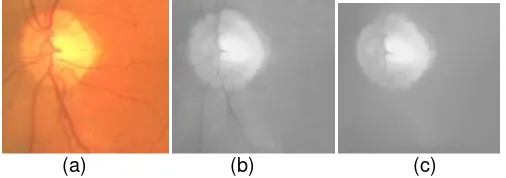
The segmentation method was tested on the DRIVE database which is available on the internet. The images are cropped to size 185 x 172 pixels. Before segmentation, the images are preprocessed to remove the blood vessels. Fig. 2 shows an example of the removed vessels in an image. The accuracy of the experimental results are compared by using two scenarios: a. Choosing R = 45 and R = 42 for circle Hough transform.
b. Choosing active contour parameter α = 10, α = 1, and α = 0.1.
The radius values significantly affect the segmentation results. The accuracy result for R = 45 is 80.18% and for R = 42 is 83.45%, for the image showed in Fig.3 and Fig, 4. The value of α affects the SPF function of the active contour. For the image showed in Figure 5 and Figure
7, the accuracy is 82.35% for α=0.1, 85.99 % for α=1, and 86.73% for α=10. The results show
that expanding the contour by increasing the balloon force α, gives better accuracy.
(a) (b) (c)
(a) (b) (c)
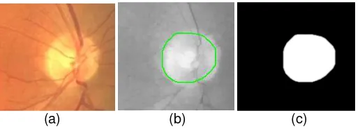
Figure 3. Segmentation result for R = 45: (a) input image; (b) contour; (c) binary mask
(a) (b) (c)
Figure 4. Segmentation result for R = 42: (a) input image; (b) contour; (c) binary mask
(a) (b) (c)
Figure 5. Segmentation result for α= 0.1: (a) input image; (b) contour; (c) binary mask
(a) (b) (c)
Figure 6. Segmentation result for α = 1: (a) input image; (b) contour; (c) binary mask
(a) (b) (c)
Figure 7. Segmentation result for α = 10: (a) input image; (b) contour; (c) binary mask
4. Conclusion
algorithm in each step should be done in order to be able to segment the cup and also to classify the abnormality such that the glaucoma diagnosis can be done automatically.
Acknowledgement
The authors would like to thank the DRIVE project team for making their image databases available on the Internet. This work was supported in part by Sepuluh Nopember Institute of Technology (ITS) under Grant 0750.254/I2.7/PM/2011.
References
[1] Quigley H A. Number of People With Glaucoma Worldwide. British Journal of Ophthalmology. 1996; 80: 389-393.
[2 ] Michelson G, Wärntges S, Hornegger J, Lausen B. The Papilla as Screening Parameter for Early Diagnosis of Glaucoma. Dtsch. Arztebl. Int. 2008; 105(34–35): 583–589.
[3] Hoffmann EM, Zangwill LM, Crowston JG, Weinreb RN. Optic Disk Size and Glaucoma. Survey of Ophthalmology. 2007; 52(1): 32-49.
[4] Chrástek R, Wolf M, Donath K, Niemann H, Paul D, Hothorn T, Lausen B, Lammer R, Mardin C, Michelson G. Automated Segmentation of the Optic Nerve Head for Diagnosis of Glaucoma. Medical Image Analysis. 2005; 9(4): 297-314.
[5] Bock R, Meier J, Nyúl LG, Hornegger J, Michelson G. Glaucoma Risk Index: Automated Glaucoma Detection From Color Fundus. Medical Image Analysis. 2010; 14(3):471-481.
[6] Welfer D, Scharcanski J, Kitamura CM, Pizzol MMD, Ludwig LWB, Marinho DR Segmentation of the Optic Disk in Color Eye Fundus Images Using an Adaptive Morphological Approach. Computers in Biology and Medicine. 2010; 40(2): 124-137.
[7] Patton N, Aslam TM, MacGillivray T, Deary IJ, Dhillon B, Eikelboom RH, Yogesan K, Constable IJ. Retinal Image Analysis: Concepts, Applications and Potential. Progress in Retinal and Eye Research. 2006; 25(1): 99-127.
[8] Winder RJ, Morrow PJ, McRitchie IN, Bailie JR, Hart PM. Algorithms for Digital Image Processing in Diabetic Retinopathy. Computerized Medical Imaging and Graphics. 2009; 33: 608–622.
[9] Niemeijer M, Abràmoff MD, Ginneken BV. Fast Detection of the Optic Disc and Fovea in Color Fundus Photographs. Medical Image Analysis. 2009; 13: 859–870.
[10] Welfer D, Scharcanski J, Marinho DR. A Coarse-to-Fine Strategy for Automatically Detecting Exudates in Color Eye Fundus Images. Computerized Medical Imaging and Graphics. 2010; 34: 228– 235.
[11] Image Sciences Institute. 2010. DRIVE: Digital Retinal Images for Vessel Extraction. Available on: URL: http://www.isi.uu.nl/Research/Databases/DRIVE .
[12] Saputra PY, Tjandrasa H. Dental Bitewing X-ray Image Segmentation for Determining the Types of Teeth, Proceeding of The 6th International Conf. on ICT and Systems. Surabaya. 2010: II-7 – II-14. [13] Djajadi A, Laoda F, Rusyadi R, Prajogo T, Sinaga M. A Model Vision of Sorting System Application
Using Robotic Manipulator. TELKOMNIKA. 2010; 8(2): 137-148.
[14] Arnia F, Pramita N. Enhancement of Iris Recognition System Based on Phase Only Correlation. TELKOMNIKA. 2011; 9(2): 387-394.
[15] Alfiansyah A. A Unified Energy Approach for B-Spline Snake in Medical Image Segmentation. TELKOMNIKA. 2010; 8(2): 175-186.
[16] Zhang K, Zhang L, Song H, Zhou W. Active Contours With Selective Local or Global Segmentation: A New Formulation and Level Set Method. Image and Vision Computing. 2010; 28: 668–676.