Synchronization Model of Traffic Light at Intersection with Train Track

(1)

Synchronization Model of Traffic Light

at Intersection with Train Track

Tomi Tristono

#

, Setiyo Daru Cahyono

*

, Sutomo

+

, Pradityo Utomo

#

Department of Management Informatic *

Department of Civil Engineering +

Department of Mechanical Engineering

University Merdeka Madiun, Madiun, East Jawa, Indonesia

[email protected], [email protected], [email protected], [email protected]

Abstract

—

The most common role of traffic lights are as signal systems to control transportation at urban networks and traffic management. Urban traffic lights in most of countries used fixed time. The traffic light systems installed on urban traffic network at an intersection consist of four arms. There is a railroad crossing on the south arm. At this time introduced the new model design of interruptive traffic lights. The new model is the syncronization between traffic lights and train doorstop. It is modeled by Petri Net. The method to analyze the model using: 1. Invariant Method. 2. Occurrence Graph Method, and 3. Simulation. The queue of vehicles happens at extension schedule less than queue at regular schedule if the closure of the railway doorstop ended when the lights north-south traffic lights red. Probability of north–south traffic light flashed red in a cycle is 0.62. The statistical expectation value of the number of queues of vehicles on extension schedule decreased. On south arm down 2.71 PCU and on northern arm down 2.34 PCU. It means that extension schedule gives positive results. The extra green 16 seconds will improve the performance of traffic light.

Key words - Synchronization, traffic light, petri net, intersection, train stop door.

I. INTRODUCTION

The most common role of traffic lights are as signal systems to control transportation at urban networks and traffic management. On traffic signal systems always integrated in two main control reasons i.e. safety and efficiency planning [1]. The main goals of its are used to manage conflicting requirements for sharing of road space, mainly often at intersection to make trip schedule by allocating right way to different sets of traffic movements during the distinct time intervals [2].

The signal systems based on time strategies has classified in two main classes [3]: 1. Fixed time systems and, 2. Traffic response systems. First, the strategy of fixed time signal system based on historical data. This is the implementation of the control signal system on simple way. The settings assume that the demand are constant, and it cannot be influenced by special events or weather conditions. Second, traffic response systems are the real time systems. Its system uses real time measurements gather by detectors located on the intersections. The detectors will give information the real conditions of demand to controllers. The controller can send messages to traffic signals to change the

duration of green or red time [4]. Urban traffic lights in most of countries used fixed time systems until today [2].

The traffic light systems installed on urban traffic network at an intersection consist of four arms. It is the left-hand traffic. It means that the traffic movement keeps on the left side of the road. There is a railroad crossing on the south arm. The presence of train to cross south arm of intersection will arise as an obstacle of the traffic movement [5]. In this event the south–north, east turn left traffic flow must stop until train finishes crossing. They must stop although the south–north traffic lights turn on green. The control of traffic lights are still separated each other with the train stopdoor controller.

At this time introduced the new model design of interruptive traffic lights. Its new model is the syncronization between traffic lights and train stopdoor. The south–north, east turn left traffic lights will turn red, when the train is crossing south arm. If the traffic lights on east arm turn on yellow or red then this should be changed to green. Its green light will have extension time until train finishes crossing.

The behavior of a traffic lights can be modeled by Discrete Event System (DES). The system often consist of a sequence of events occur at specific instants of time [6]. DES can present the relationship between environment, conflict of resources and occurrence of activities. We use DES to make the design of the traffic light systems. The model DES is expressed by Timed Place Petri Net (TPPN). TPPN are suitable to model traffic light systems because they offer representation of conflict situations, share resources, synchronous and asynchronous communications, and precedence constraints [4].

II. BASIC DEFINITION OF PETRI NET

Petri Net (PN) has proven to be a powerfull technique for solving many kinds of difficult problems associated with modeling, formal analysis, design and coordination control of discrete event systems [7]. Major advantage of Petri Net is the model can be used for the analysis of behaviorial properties and performance evaluations [8]. The basic Petri net is composed of four-tuple elements: places, transitions, arcs and tokens [6].

(2)

circles and transition by bars. The Basic definition of a Petri net structure [4] is given as follows:

Definition 1. A Petri net structure is a four-tuple elements N=(P, T, Pre, Post).

P = {p1, p2, p3, . . . pn} is the finite set of places, P

z

׎, T = {t1, t2, t3, . . . m} is the finite set of transitions, T

z

׎, Pre : (PxT)

o

N+ is an input function that defines directed arcs from places to transitions, Post : (TxP)

o

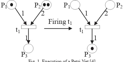
N+ is an output function that defines directed arcs from transitions to places and N+ is the set of nonnegative integers.

Fig. 1 is the representation of a Petri net and the execution. Initial places are P1 and P2. Places P1 consist of two tokens and P2 consist of one token. The transition t1 is enabling. After the firing of transition t1, the tokens in places P1 and P2 are removed, and one token is deposited in place P3, as the weight of the arc from t1 to P3 is one.

Definition 2. A Petri net is a two-tuple PN = (N, M0), wherePN is a Petri net, and M0 is the initial marking.

It dynamic behavior is described by markings from M0 to Mn, which is indicated by firing of an enable transition. A transition t

T is enable if any places p

P as an input arc t contains at least the numberof tokens equal to the weight of the arcs connecting p to t(M(p) ≥Pre(p,t) for any p

P)

III.PROPERTIES OF PETRI NET

It is very important that the design models are correct. Another definition of correct models is indicated by a set of desirable properties. These allow the designers to identify the presence or absence of functional properties [4]. The most common ones are:

a. Reachability: In a Petri Net, transition firing will result in a sequence of markings that are reached with the change of token distribution. A marking of Mn is said to be reachable

from a marking Mo if there exists a sequence of firing that

that transform from Mo to Mn. This is denoted by R(N,M0).

The problem is finding the sequence marking that Mn

R(N,M0).

b. Reversibility: In a reversible Petri Net, it is always possible to return to the initial marking or state.

c. Boundedness: A Petri Net (N, Mo) is k-bounded if the number of tokens in each place does not exceed k for any marking reachable from Mo , k is a nonnegative integer.

d. Safeness: A Petri Net (N, Mo) is said to be safe if it is 1-bounded [7].

e. Liveness: A Petri Net (N, Mo) is live if for every marking M that can be reached from Mo. A live Petri Net

guarantees deadlock free operation [4].

P

1

P

2

P

1

P

2

1 2 1 2

Firing t

1

t

1

t

1

1 1

P

3

P

3 Fig. 1. Execution of a Petri Net [4].

IV. TIMED PLACE PETRI NET.

Events modelled by Petri Net will have an event time. The Timed Place Petri Net [9] adds time interval to each place.

Definition 3. A Timed Place Petri Net is a pair (PN, Ip). PN is a Petri Net and Ip is defined as

Ip : P

o

(Q+

0)x(Q+

f

).

Each place p

P have a timed interval Ip=(α, β) is

associated with 0 ≤α≤β. Ip is time interval as duration which

a token available at place p.

The east traffic lights at Fig. 2 are modeled by places GE (Green East), YE (Yellow East), RE (Red East), transition t7, t8, and t9. There are six arcs i.e. as three input fuction and also three output function of transitions. The weight of every arcs in this timed model are equal with one and it unnecessary written. A token exists at place GE, it means that the green light is turn on. A token available at place GE with duration

[τ3, τ4]. Transition t8 will enable to fire after duration of place GE has finished. The firing of transition t8 will remove a token from place GE to place YE. A token available at place

YE with duration [τ4, τ5]. It means that the yellow light will

turn on. Transition t9 will enable to fire if the duration of YE has been at full time. A token will remove to place RE and red

light turns on. The its duration is [τ5,τcycle] + [τ0,τ3]. They both are full duration of RE. The first part of the time interval is

starting from τ5 and the ending at the full time of a cycle τcycle.

Next, the Petri Net will reversible to initial marking with

duration [τ0,τ3]. Its additional time will start after duration of

a cycle finishes without delay time.

Definitions 4. A Petri Net Componen is a tuple PNC = (PN, IP, OP).

PN is Petri Net, IP={Ip1, Ip2, Ip3, … , Ipn}

P is the set of input places, and OP={Op1,Op2,Op3,…, Opn}

P is the set of output places.

Definition 5. An Interface of a Petri Net Componen IPNC is the union of set IP and OP.

IPNC = IP

OP.

IPNC connected real world with places of PN.

t7

GE [τ3, τ4] t8

YE [τ4, τ5]

t9

RE [τ5,τcycle]+ [τ0,τ3]

(3)

V. MODEL OF TRAFFIC LIGHT

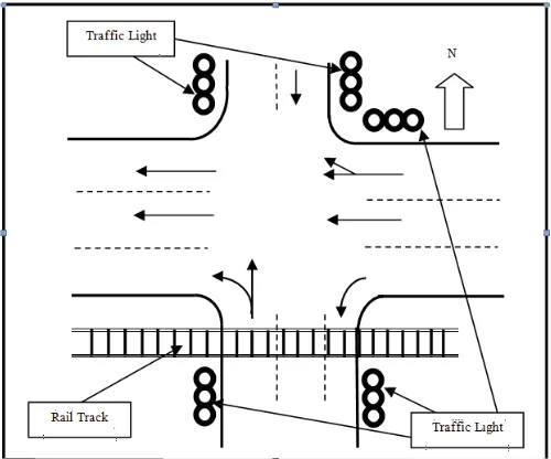
The detail information of signalized intersection as follows: Fig. 3. is map the real conditions of intersection. Its the left-hand traffic. It means that the traffic movement keeps on the left side of the road. The streams approach from east arm of intersection move on one direction to west. They will go stright to west arm, turn right to north arm, and go to south arm with Left Turn on Red (LTOR). The traffic from south and north arms move on two directions i.e. its approching and vehicles moving away from the intersection. Traffic comes from north is allowed to go straight to south arms only and they are prohibited to turn right although traffic light turn on the green light.

The stream of vehicles from south is allowed to go straight and turn left. The traffic at west arm moves on one direction and keep away from the intersection.

The Schedule of traffic lights systems are installed on fixed time, and its consist of two phases only. Phase 1 is phase_NS (North–South) and phase 2 is phase_E. (East) [10]. The definition of a cycle in each phase of regular traffic light system is represent duration of green period, yellow, and red. Phase_NS and phase_E have the same duration of one cycle.

The eastern arm is the main road while the north-south arm of the minor road. volume of vehicles crossing the main road is also higher when compared to the volume on the minor road. consequently the duration of the green on the east arm is always greater than the duration of the green on the north south. Vehicle on the main road is dominated by heavy vehicles (HV) and passenger vehicles or low vehicles (LV), while the minor roads are dominated by passenger vehicles (LV) and motorcycles (MC) [10].

The other assumptions made in this model is that no pedestarian signals exist. This of course does not mean that their flows do not exist, but they are referred to use vehicle signal indications.

The models of traffic lights using petri net is constructed in next Fig. 4.

Fig. 3. the intersection with train rail tracks at one arm.

TABLE 1. ORIGINAL AND DESTINATION

Phase Phase NS Phase E

Original south arm north arm east arm Destinations are

allowed

north arm & west arm

south arm south, west & north arm Direction

Stream

N

TABLE 2.

DURATION OF A TRAFFIC LIGHT

Phase Green Inter Green Red Cycle Yellow All red

Phase

NS [τ0 ,τ1] [τ1, τ2] [τ2, τ3] [τ2 ,τcycle] [τ0, τcycle] Phase

E [τ3, τ4] [τ4, τ5] [τ5, τcycle]

[τ5 ,τcycle] +

[τ0, τ3]

[τ3, τcycle]

τ0 < τ1 < τ2 < τ3 < τ4 < τ5 < τcycle , τ0 = 0, τi

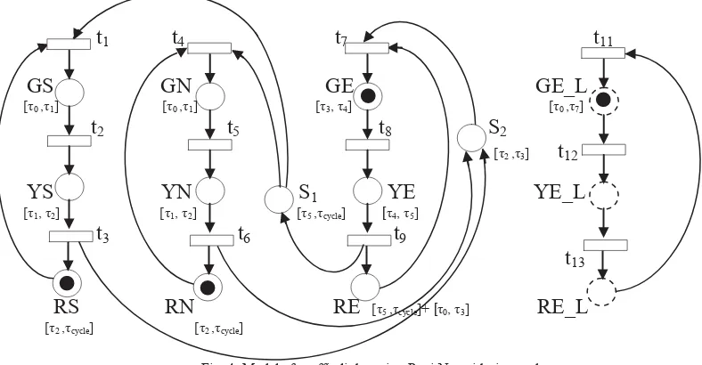
N+

The regular traffic light is modeled as places GS (green south), YS (yellow south), RS (red south), GN (green north), YN (yellow north), RN (red north), GE (green east), YE (yellow east), RE (red east), GE_L (green east turn left), YE_L (yellow east turn left), and RE_L (red east turn left). S1 and S2 are the intermediaries to make time order phase 1 (phase North-South) and phase 2 (phase East). Phase NS consist of places of traffic lights GS, YS, RS at south arm, GN, YN, and RN at north arm. Traffic light at south arm and north arm turn on same color simultanously. Phase E (east) consist of places of traffic lights GE, YE, and RE. The traffic lights east turn left consist of GE_L, YE_L, and RE_L. It is the virtual traffic lights. This traffic does not exist at the real world. The traffic lights of vehicles come from east to go to south arm will do left turn on red (LTOR). It means that the traffic light as if always turn on green. The yellow light will turn on if the controller has sent a message. The next, it will turn on red. The duration of red light (RE_L place) depends on the time interval of closing train doorstop.

Fig. 4. indicates that a token in the each places RS and

RN with duration [τ2 ,τcycle] and place GE with duration [τ3,τ4].

GE_L has green duration [τ0, τ7], and with τ7 = ∞. It means

that if red light turn on in phase NS then the green light turn on in phase E. Where τi

N+ is an element of the set of positive integers.

In general, initial state of traffic light model τ0 = 0. It starts from the traffic light turns green, but this is not absolute. It is based on cycles of continuous traffic lights then initial state of traffic lights can also be started from the yellow or red.

VI.ANALYSIS OF TRAFFIC LIGHT

(4)

t

1

t

4

t

7

t

11

GS GN GE GE_L

[τ0 ,τ1] [τ0 ,τ1] [τ3, τ4] [τ0 ,τ7]

t

2

t

5

t

8

S

2

[τ2 ,τ3]

t

12

YS YN S

1

YE YE_L

[τ1, τ2] [τ1, τ2] [τ5 ,τcycle] [τ4, τ5]

t

3

t

6

t

9

t

13

RS RN RE

[τ5 ,τcycle]+ [τ0, τ3]

RE_L

[τ2 ,τcycle] [τ2 ,τcycle]

Fig. 4. Model of traffic light using Petri Net with time order.

The three methods to analyze the properties Petri net are: 1. Invariant Method. 2. Occurrence Graph Method, and 3. Simulation [2].

A. Invariant.

The marking of a Petri net can be presented by the firing of enable transitions. All reachable markings have some common properties. The properties guarantee that they will not vary when the transitions are fired, it is said to be invariant equations.

GS+YS+RS=1 (1)

The invariant at (1) asserts that it can be only a token available in one of three places GS, YS, and RS. It also indicates that the sequence of event to be in time order at south traffic light.

GN+YN+RN=1 (2).

GE+YE+RE=1 (3).

GE_L+YE_L+RE_L=1 (4).

The next invariant at (5) indicates that if there is a token in place RE, then there must be a token in either place GS, YS, or RS. It means that once the red signal goes on in the east traffic light for vehicles go straight and turn right, then a green, a yellow, or a red signal must be turned on in the south traffic light. Its provided to the traffic vehicles come from south to go to north direction or turn left.

GS+YS+RS=RE where RE=1 (5).

In other way with the next invariant.

GN+YN+RN=RE where RE=1. (6).

GE+YE+RE=RS where RS=1 (7).

GE+YE+RE=RN where RN=1 (8).

GE_L =1 (9).

The next invariant is equipped with intermediation places S1 and S2.

GS+YS+GE+YE+S1+S2=1. (10). GN+YN+GE+YE+S1+S2=1. (11)

As previously mentions in (10)-(11), these invariant mean that the direction of the vehicles movement. These invariant hints that the models system guarantee the safety of traffic.

All equations from (1)–(11) present the key invariant in Petri net model system. They show the model system is invariant.

B. Occurrence Graph.

The idea behind occurrence graph (OG) is constructing a graph. It contains a node for each reachable marking and an arc for each occurring binding element. This approach can see that there is no possibility of deadlock in the model [2].

At Fig. 5. each node presents a marking and the content of the marking is described by the text of the node. The each arcs represent of occurrence of the event. For example, the text YS, YN, RE, and GE_L are use to describe node N1. It means that the yellow light at south arm and north arm turn on. The traffic light at east arm for vehicles will turn right and go straight turn on red light. The traffic from east turn left always turn on green light.

N0 N1 N2

T1 T2

T6 T3 N5 N4 N3

T5 T4

Fig. 5. the Occurrence Graph Petri Net Model RS, RN

YE, GE_L

[τ4 ,τ5] S1

RS, RN RE, GE_L

[τ5 ,τcycle]

RS, RN GE, GE_L

[τ3 ,τ4] S2

RS, RN RE, GE_L

[τ2 ,τ3] Initial

GS, GN RE, GE_L

[τ0 ,τ1]

YS, YN RE, GE_L,

(5)

GS YS- _RS

GN YN _RN

S2

RE GE YE

GE_L

S1

τ

0

τ

1

τ

2

τ

3

τ

4

τ

5

τ

cycle time

Fig. 6. Simulation results of Regular Schedule.

All traffic lights at node N1 will have duration [τ1 ,τ2]. After firing T2, they will change to node N2.

C. Simulation.

Simulation of traffic lights the Petri net using computer software applications. The simulation made with both advanced timed place petri net and basic petri net without attached time interval. The duration basic model of traffic light is presented by an amount of tokens in the places. It means that each token is attached time stamps. For example, the place GS with nine tokens, it means that the traffic light has a remaining nine seconds to light up. The tokens must be fired one by one until they are run out and eventually the place GS will be empty. The arcs are connecting each places have different weight. If the green light at south arm has a duration twenty-nine seconds then the input arc must also have the same amount of weight [11]. The model has fulfilled all petri net properties and there was no deadlock, but it was more complicated than model Timed Place Petri Net. Here only present the results of the simulation models.

VII. MODEL EXTENSION OF TRAFFIC LIGHT SYSTEM. Extension schedule model is the petri net model connected with real world. It uses sensors. The sensors will detect and send messages that has been present a train on the railroad. First, The actual messages would be processed at traffic light control systems. This event causes the stream of vehicles from south, north, and east will turn left must stop. The extention scheduling of trip will be interrupted regular schedule. It bases from the instruction of traffic light control systems. The extention schedule model using petri net presented that south – north and east turn left traffic lights must be turned on red, and the east arm turned on green. The green signal on east arm provided for the vehicles to go straight and turn right. It will have time extension until train finished crossing the south arm. After this event is completed then the traffic lights south, north, and east turn left will turn on green with regular schedule.

A. Invariant Method of Extension Schedule.

In these next equations are defined that the traffic light extention is written by extension (ext), for example RSext is traffic light on south turn on at extension time.

GS+YS+RSext =1 (12)

The invariant at (12) asserts that it can be a token only available in one of three places GS, YS, and RSext. It also indicates that the sequence of event to be in time order at

south traffic light. Initial time order starts at RSext, RNext, and RE_Lext.

GN+YN+RNext =1 (13).

GEext +YE+RE=1 (14).

GE_L+YE_L+RE_Lext =1 (15).

The invariant (16) indicates that if there is a token in place RE, then there must be a token in either places GS, YS, and RSext.

GS+YS+RSext =RE where RE=1 (16).

In other way with the next invariant equations.

GN+YN+RNext =RE where RE=1. (17).

GEext +YE+RE=RSext where RSext=1 (18).

GEext +YE+RE=RNext where RNext=1 (19).

RE_L = RSext =RNext = Train_DoorStop (20). The next invariant at extention time is equipped with intermediation places S1 and S2.

GEext+YE +S1+GS+YS+S2=1. (21).

GEext +YE+S1+GN+YN+S2=1. (22).

As has been mention above in (21) and (22), these invariants hints that the models systems guarantee the safety of traffic. All equations from (12)–(22) has presenting the invariant in Petri net model system. The model system is invariant.

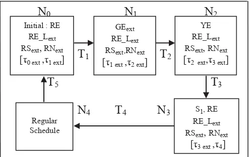
B. Occurrence Graph of Extention Schedule.

The occurence graph at extention time schedule as follows at Fig. 7.

C. Simulation of Extention Schedule.

The simulations have been performed using computer software applications. The simulation made with timed place petri net. It means each place models have time durations.

N

0

N

1

N

2

T

1

T

2

T

5

T

3

N

4

T

4

N

3

Fig. 7. the OG Petri Net Model of Extention Schedule. Regular

Schedule

S1, RE RE_Lext RSext, RNext

[τ3 ext ,τ4] YE RE_Lext RSext, RNext

[τ2 ext,τ3 ext] Initial : RE

RE_Lext RSext, RNext

[τ0 ext ,τ1 ext]

GEext RE_Lext RSext,RNext

(6)

RSext GS YS RS

RNext GN YN RN

S1

RE GEext YE RE GE

RE_Lext GE_L

S2

τ

0 ext

τ

1 ext

τ

2 ext

τ

3 ext

τ

4

τ

5

τ

6

τ

7

time Fig. 8. Simulation Result with Extension Schedule.

The duration of the extention depends on schedule closing time interval doorstop railroad crossing. The models satisfy all properties of petrinet i.e. safe, life, reachable all places, and never deadlock.

VIII. QUEUE OF VEHICLES AND PROTOTYPE

Standart metric in this paper uses Passanger Car Unit (PCU). It used in transportation engineering to assess traffic flow rate on a highway. It is sometimes also used both metric Passanger Car Unit (PCU) or Passanger Car equivalent (PCE). That is the effect of traffic variables if it compared to a single passanger car. The typical values of PCU or PCE are private car, taxi, pick up (Low Vehicle/LV) equal with 1, bus, truck, trailer (High Vehicle/HV) equal with 1.3, motorcycle (MC) equal with 0.2, and unmotorized vehicle (UM) equal with 0 or it means ignored [11]. It based on observation result that the maximum capacity south arm about 700 PCU/hour, north arm about 750 PCU/hour, and the east arm about 1750 PCU/hour. Volume of traffic flow coming from south arm about 540 PCU/hour, north 470 PCU/hour, and from east 1020 PCU/hour. It is assumed that vehicles have uniform arrival function distribution. Traffic flow comes from east 15% turn left to the south arm. Degree of saturation at south arm 0.78, at north arm 0.64, and at east arm 0.58.

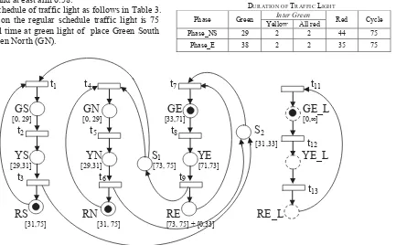
The regular schedule of traffic light as follows in Table 3. Lenght of a cycle on the regular schedule traffic light is 75 seconds. The initial time at green light of place Green South (GS) and place Green North (GN).

The simulation has happened closing train doorstop for 99 seconds. set time was approaching an average of the actual closing time. The duration of closure of the railway doorstop is almost always longer than a traffic light cycle. Closure duration shorter than the time interval a cycle is very rare because it is very dangerous to the passing vehicles.

The calculation of the number of vehicles queuing arising is based on a formula Indonesian Capasity Highway Manual [12]. We discuss the number of vehicles queuing comparisons arise between regular schedule and schedule extensions when the train crossed south arm.

Initial start of the simulation time begins when the traffic light turned red at the NS phase. Initial turn on red is also the beginning of the railway crossing the south arm. This is done so that the implementation of the simulation becomes easier .

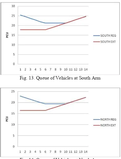
Simulation results show that the extension schedule does improve efficiency. The extension schedule indicates that the performance is better. It leads to a shorter vehicle delay and fewer stops. Comparison in detail can be seen in Table 4, whereas the image shown in Fig. 13, Fig. 14, and Fig. 15. The blue line is plot of the curve on a regular schedule (REG) and the red line is the result of a schedule extension (EXT).

TABLE 3.

DURATION OF TRAFFIC LIGHT

Phase Green Inter Green Red Cycle Yellow All red

Phase_NS 29 2 2 44 75

Phase_E 38 2 2 35 75

t

1

t

4

t

7

t

11

GS

GN GE GE_L

[0, 29] [0, 29] [33,71] [0,∞]

t

2

t

5

t

8

S

2

[31,33]

t

12

YS YN S

1

YE YE_L

[29,31] [29,31] [73, 75] [71,73]

t

3

t

6

t

9

t

13

RS RN RE RE_L

[31,75] [31, 75] [73, 75] + [0,33]

(7)

t

4

t

1

t

7

t

11

GS

GN GE GE_L

[99, 128] [99, 128] [2,95] [99,∞]

t

2

t

5

t

8

S

2

[0, 2]

t

12

YS YN S

1

YE YE_L

[128, 130] [128, 130] [97, 99] [95, 97]

t

3

t

6

t

9

t

13

RS RN

[0, 99]

RE RE_L

[0, 99] [0, 99] [97, 132]

Fig. 10. Model of traffic light using PN with Extension Time 99 seconds.

N0 N1 N 2

T1 T2

T5 T3

N4 N3

T4

Fig. 11. The OG PN Model with Extention Time 99 second.

Petri net model shown in Fig. 10. is scheduling extension with an extension to 99 seconds the red light on the phase of NS.

There is a token in the GE. This means that the traffic lights for vehicles from the east arm turns green. This signal is provided for a vehicle that will go straight to the west and turn right into the north arm. The duration is for 93 seconds. This starts from 2nd to 99th seconds. It presented at Fig. 11 on N1.

There is a token on each RS places, RN, and RE_L. This means that vehicles from the north, south, and east turn left must stop. The duration is 99 seconds, the same time interval with the closure of the railway doorstop.

At the end of the extension schedule will be left back to regular schedule when the railway was completed across the southern arm. The beginning of the regular cycle starts with a green signal in phase NS. There is no time delay on the order of traffic lights turn on the extension schedule to the regular schedule originally.

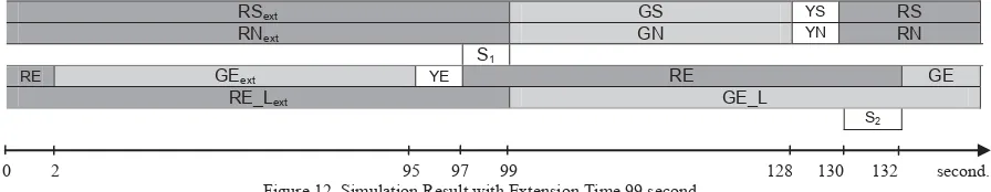
In Fig. 11. appears Occurrence graph on extension schedule only. It will return to regular schedule, after the occurence in N3. The simulation results shown in Fig. 12.

The number of vehicles stopped due to the closure of the railway doorstop is as follows:

The number of vehicles stopped on the east turn left reaches 4.2 PCU. This has not changed either on a regular schedule and extension schedule.

The saturation degree of the traffic from east to go straight and turn right at extension schedule 0.41. It is lower than the saturation degree at regular schedule

The average vehicle stops on a regular schedule and comes from the south is 22.72 PCU while those from the north, ie 20.62PCU.

RSext GS YS RS

RNext GN YN RN

S1

RE GEext YE RE GE

RE_Lext GE_L

S2

0 2 95 97 99 128 130 132 second.

Figure 12. Simulation Result with Extension Time 99 second. Regular

Schedule

S1, RE RE_Lext RSext,RNext

[97, 99] YE RE_Lext RSext, RNext

[95, 97] Initial : RE

RE_Lext RSext, RNext

[0, 2]

GEext RE_Lext RSext, RNext

(8)

TABLE 4. TOTAL VEHICLES STOP.

Number

Start

at Began at (second)

Vehicles Stop at Regular Schedule Vehicles Stop at Extension Schedule

Stop (second).

Final Stop at

South (PCU)

North (PCU)

Stop (Second)

South (PCU)

North (PCU) 1 Green

Light

5th ₁₄₅ _red _25.38 _22.92 ₁₀₀ _17.80 _16.36

2 10th ₁₄₀ _red _24.52 _22.17 ₁₀₀ _17.80 _16.36

3 15th ₁₃₅ _red _23.65 _21.43 ₁₀₀ _17.80 _16.36

4 20th ₁₃₀ _red _22.79 _20.68 ₁₀₀ _17.80 _16.36

5 25th ₁₂₅ _red _21.93 _19.94 ₁₀₀ _17.80 _16.36

6 Red

Light

0 120 red 21.24 19.34 100 17.80 16.36

7 5th ₁₂₀ _red _21.24 _19.34 ₁₀₅ _18.66 _17.10

8 10th ₁₂₀ _red _21.24 _19.34 ₁₁₀ _19.52 _17.85

9 15th ₁₂₀ _red _21.24 _19.34 ₁₁₅ _20.38 _18.59

10 20th ₁₂₀ _green _21.24 _19.34 ₁₂₀ _21.24 _19.34

11 25th ₁₂₅ _green _22.10 _20.09 ₁₂₅ _22.10 _20.09

12 30th ₁₃₀ _green _22.97 _20.83 ₁₃₀ _22.97 _20.83

13 35th ₁₃₅ _green _23.83 _21.58 ₁₃₅ _23.83 _21.58

14 40th ₁₄₀ _green _24.69 _22.32 ₁₄₀ _24.69 _22.32

The average vehicle stops on the schedule extension and comes from the south is 20:01 PCU while those coming from the north is 18:28 PCU.

The duration of the extension schedule and regular schedule has a significant time difference. this case if the opening of the railway doorstop occurs when the north-south traffic lights flashed red. The duration of the red traffic light for north-south arm is 44 seconds. duration of a cycle is 75 seconds. So the probability of glowing color red is 44/75 or equal to 0.62. Statistical expectation value of the queue of vehicles has decreased. The decline in the southern arm is at 2.71 PCU, while the north arm 2.34 PCU. It means that extension schedule always give positive result.

Fig. 13. Queue of Vehicles at South Arm

Fig. 14. Queue of Vehicles at North Arm

Fig. 14. Time Stop

TABLE 5.

THE NUMBER OF CYCLES NEEDED TO RESOLVE VEHICLES CONGESTION

North-South Green Duration

Vehicles Congestion Caused by Closure of The Railway Doorstop

Only

Return to The Initial Degree Of Saturation (Vehicles Congestion

Caused by Closure of The Railway Doorstop & arrival) South

Arm (cycles)

North Arm (cycles)

South Arm (cycles)

North Arm (cycles) On the

regular Schedule

4 3 16 10

On the first green with 16 seconds of extra time

3 2 10 5

Degree of saturation in the east arm when the train passes is 0.35. This value when scheduling at first green with 16 seconds of extra time, it will reach 0.63 . This value is higher than the degree of saturation on a regular schedule, that is 0.58. At a later stage the degree of saturation will be down close to 0.58.

(9)

circuit (IC). It contains processor core, memory, and programmable input/ output. Microcontroller is designed for single embedded system. Red, yellow, and green signals using light emitting diode (LED). The sensor devices system uses the invisible light, infrared. If the sensor devices detect the presence of the train then they will send messages to microcontroller. The microcontroller instructs train doorstop to close and the schedule for the sequence of traffic lights to adjust with them. This situation occurs in emergency situations only. Finally, the proposal of modeling framework can be applied to a intersection. It will increase the safety and fair time sharing to the traffic stream.

IX.CONCLUSION.

The extension schedule of traffic light has been modeled by Petri Net. The time stop in extension schedule less than or equal with that which one in regular schedule. The consequences of the time stop is arising the queue of vehicles. The queue of vehicles arise in extension schedule less than or equal with that which one in regular schedule. Total amount depends on the final closing doorstop. If the final of closing doorstop occurs when north–south traffic light turn on red then it will arise lower number of queues of vehicles. If it occurs when north–south traffic light turn on green or yellow, the number of queues of vehicles which arise similar to those seen on a regular schedule. This can be seen in theFig. 13 and Fig. 14 above. Probability of north–south traffic light turn on red in a cycle is 0.62. Statistical expectation value of the vehicle queue at the south arm of the extension schedule PCU 2.71 lower than that on a regular schedule and that in the northern arm on extension schedule 2.34 PCU lower than that on a regular schedule. It means that extension schedule gives positive results. The first green on the north-south phase is when the train was finished passing changed. Its duration plus 16 seconds of extra time. This will improve the performance of traffic light.

ACKNOWLEDGMENTS.

This research is funded by the Directorate General of Higher Education (DGHE) with scheme Competitive Grant (Hibah Bersaing) in 2014.

REFERENCES.

[1] ITE, Traffic Engineering Handbook, 6th Edition Institution of Trasportation Engineers, 2009.

[2] Huang,YS and Chung, TH, “Modelling and Analysis of Traffic Light Control Systems Using Timed Colored Petri Net”, Intechopen.com, 2010.

[3] Papageorgiou,M., Diakaki, C., Dinopoulou,V.,

Kotsialos,A., Wang,Y., “Riview of Road Traffic Control Strategies”, Proceedings of IEEE., pp. 2043-2067, 2003.

[4] Soares, M, “Architecture-Driven Integration of Modeling

Languages for the Design of Software-Intensive Systems”, Thesis, Published and distributed by: Next Generation Infrastructures Foundation, Delft The Netherlands, Chapter 7, pp 99-133, February 2010.

[5] Hutauruk, S.,Gulo, N., “Mengurai Kemacetan

Lalu-Lintas pada Area Lalu-Lintasan Kereta Api yang Berdekatan dengan Simpang Empat”, Prosiding Seminar Nasional Teknologi Informasi & Komunikasi Terapan 2012 (Semantik 2012), ISBN 979-26-0255-0, Semarang, Juni 2012.

[6] Cassandras, CG., Lafortune, S., “Introduction to

Discrete Event Systems”, The International series on

Discrete Event Dynamic Systems, Kluwer Academic Publisher, Norwell, Massachusetts, USA,1999.

[7] Murata, T., “Petri Net: Properties, Analysis, and Applications”, Proceedings of IEEE, vol 77, pp 541 -590,1989.

[8] Tianlong, GU., Parisa, AB., Guoyong,CAI., “Timed

Petri Net Based Formulation and An Algorithm for The Optimal Schedulling of Batch Plants”, Int. Journal Applied Mathemathics and Computer Science, vol 13, No 4, pp 527-536, 2003.

[9] Khansa, W., Aygaline, P., Denat, J., “Structural Analysis of P-Time Petri Nets”. In: Symposium on Discrete Events and Manufacturing Systems, Proceedings of the CESA'96 IMACS Multiconference, 1996.

[10] Tristono, T., “Study of Traffic Vehicles on Signalized

Intersection with Train Track Using Graf Model”,

Journal Agritek, vol 15, ISSN 1411 5336, University Merdeka Madiun, pp 81-91, March, 2014.

[11] Adzkiya, D., Subiono., “Modelling Traffic Light Using

Petri Net and Its Simulation”, Thesis, Institut Teknologi

Sepuluh Nopember, Unpublished, Surabaya, 2008.

[12] ICHM, “Indonesian Capasity HighwayManual (MJKI)”,