Development of a Free-Free Transverse Beam Model Using Lateral
Vibrations of Beam Conventional Method during Seismic Activity
M.A. Salim
Faculty of Mechanical Engineering, Universiti Teknikal Malaysia Melaka Hang Tuah Jaya, 76100 Durian Tunggal, Melaka, Malaysia
E-mail: [email protected] A. Noordin
Faculty of Electrical Engineering, Universiti Teknikal Malaysia Melaka Hang Tuah Jaya, 76100 Durian Tunggal, Melaka, Malaysia
E-mail: [email protected] M.Z. Akop
Faculty of Mechanical Engineering, Universiti Teknikal Malaysia Melaka Hang Tuah Jaya, 76100 Durian Tunggal, Melaka, Malaysia
E-mail: [email protected]
Received: December 16, 2010 Accepted: January 6, 2011 doi:10.5539/jmr.v3n3p77
The research is financed by Faculty of Mechanical Engineering, Universiti Teknikal Malaysia Melaka, Malaysia.
Abstract
This paper expresses the derivation of Free-Free Transverse Beam Model using lateral vibration of beam conventional method during Seismic Activity. Derivation from three mathematical models givescoshβLcosβL=1.Then by numerical software, the graph of those mathematical models is plotted. From the plots, and using equations, the natural frequencies of those three models are identified at values of 389.5 rad/s, 2440.9 rad/s, and 6825 rad/s forω1, ω2andω3respectively.
Keywords:Free-free beam, Transverse beam, Lateral, Mathematical model
1. Introduction
Vibration is mitigated as the relative motion which takes place between the structure and the mass via the dashpot. This kind of energy dissipation allows the beam to obtain some of the external force in place of the structure for stabilization. Vibration is defined as a periodic back and forth motion of the particles of an elastic body or medium. It is usually a result of the displacement of a body from an equilibrium condition, followed by the body response to the forces that tend to restore equilibrium (Shirley 1996). It is also considered as the transfer between the kinetic energy and potential energy. It means that the vibration systems have their energies both stored and released. Recently, it has been argued that vibration refers to mechanical oscillations about an equilibrium point.
before.
2. Analytical model
In this study, there are three model were developed to analyze the behavior of the free-free beam when the seismic activity happens. There are:
1. One dimensional mathematical model 2. Two dimensional mathematical model 3. Three dimensional mathematical model
All of these three mathematical models were derived and are shown in equation 1 till equation 23 below. <Figure 1>
The initial boundary condition of this free-free beam isx=0 when the distance is defined at the left point andx=Lwhen the boundary is taken from the right point.
The one dimensional mathematical model can be derived by using the equation 1 below: dy
dx=0 (1)
Two dimensional mathematical models can be stated derived by using equation 2. d2y
d2x =0 (2)
And three dimensional mathematical models can be derived by using equation 3. d3y
d3x =0 (3)
By using the equation of wave propagation in beam, the initial equation of free-free beam can be stated in equation 4.
y=Asinhβx+Bcoshβx+C sinβx+Dcosβx (4)
Then, equation 4 was applied to the equation 1, 2 and 3 and the new equations are shown in equation 5, 6 and 7. dy
The initial boundary condition ofx=0 was set and the boundary condition was applied into the equation 6. The free-free beam equation then was changed to the novel equation of free-free transverse beam and is shown in the equation below.
d2y
Then, an assumption was made that equation 8 is equal to zero. The new equation can be expressed as equation 9 below.
β2[A(0)+B(1)−C(0)−D(0)]=0 B−D=0
The initial boundary condition is used again and for this time the boundary condition is applied into equation 7.
The same assumption is also made for equation 10. The new equation is:
β3[A(1)+B(0)−C(1)+D(0)]=0 A−C=0
A=C (11)
The boundary condition is set atx=L. This boundary condition is applied to second derivative (equation 6) of free-free transverse beam. The unknown constants of C and D are changed to A and B, respectively. The reason is to make the equation more easily to be solved accordingly. The new equation is expressed as below.
d2y dx2 =β
3[AsinhβL+BcoshβL−AsinβL−BcosβL] (12)
Then, assumption is made to equation 12, to be equal to zero.
β3[AsinhβL+BcoshβL−AsinβL−BcosβL]=0 AsinhβL+BcoshβL−AsinβL−BcosβL=0
A(sinhβL−sinβL)+B(coshβL−cosβL)=0 (13)
The same boundary condition is then applied into the third derivative (equation 7). The unknown also is changed as the same as equation 12.
d3y dx 2
=β3[AcoshβL+BsinhβL−AcosβL+BsinβL] (14)
An assumption is made to equation 14 to be equal to zero. The new equation can be expressed by the equation below.
β3[AcoshβL+BsinhβL−AcosβL+BsinβL]=0 AcoshβL+BsinhβL−AcosβL+BsinβL=0
A(coshβL−cosβL)+B(sinhβL+sinβL)=0 (15)
The equations 13 and 15 were rearranged into matrix form. The purpose of this matrix form is to identify the governing equation of free-free transverse beam. Besides that, matrix form is used to represent the equations into more simple form. The matrix form of the equations can be represented as below.
Equation 10 and 12 in matrix form is:
(sinhβL−sinβL) (coshβL−cosβL) (coshβL−cosβL) (sinhβL+sinβL)
A Then, the equation 16 is rearranged to solve the governing equation of free-free transverse beam.
(sinhβL−sinβL)(sinhβL+sinβL)−(coshβL−cosβL)(coshβL−cosβL)=0
[(sinh2βL)+(sinhβLsinβL)+(−sinβLsinhβL)+(−sin2βL)]
sinh2βL+sinhβLsinβL−sinβLsinhβL−sin2βL
−cosh2β+coshβLcosβL+cosβLcoshβL−cos2βL=0 (18)
sinh2βL−sin2βL−cosh2βL+coshβLcosβL+cosβLcoshβL−cos2βL=0 (19) sinh2βL−sin2β−cosh2βL+2coshβLcosβL−cos2βL=0 (20) The trigonometric identity is applied in Equation 20 in order to solve it.
The new equation of free-free transverse beam is shown in equation 23: 2coshβLcosβL=2
coshβLcosβL=1 (23)
3. Results and discussion
Based on the one, two and three dimensional mathematical models, there are three graphs can be plotted and they are: 1. First mode shape
2. Second mode shape 3. Three mode shape
The natural frequency equation is shown in equation 24.
ωn=β2
&
EI
ρA (24)
In this study, aluminum material was used because aluminum is one part of metal material. Besides, the density of this material is low but the Young Modulus E is high. According to this reason, aluminum has been chosen in this study. From the lateral vibrations of beams, the mode shape can be identified. For the first mode shape, the value ofβL=1.875104 andβ=1.8751042. Therefore, the first natural frequency is:
ω1=0.879×443.125=389.5rad/s (25)
For second mode shape, the value ofβL=4.694091 andβ=4.694091/2. The second natural frequency is:
ω2=5.5086×443.125=2440.9rad/s (26)
Lastly for third mode shape, the value ofβL=7.854757 andβ=7.8547572. The third natural frequency is:
ω3=15.4243×443.125=6825rad/s (27)
4. Conclusion
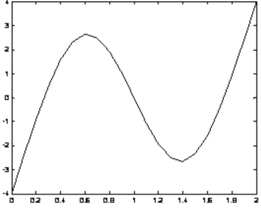
In this study, the one, two and three dimensional mathematical model from free-free beam are derived by using the lateral vibration of beams method. Based on this method, the free-free beam equation has changed to free-free transverse beam equation and the final equation iscoshβLcosβL=1. Besides that, according to this lateral vibration of beams method, the analytical analysis of first, second and third natural frequencies of the free-free beam can be identified. By using the numerical software, the graph of these three mode shapes has been shown in Figure 2. (a), (b) and (c) for the first, second and third mode shapes, respectively.
Acknowledgement
The author would like to thank to the Faculty of Mechanical Engineering, Universiti Teknikal Malaysia Melaka, Malaysia.
References
C.F. Beards. (2000).JStructural vibrations: Analysis and damping, New York, Arnold Ltd. pp 3.
J.D. Shirley. (1996). Acceleration feedback control strategies for active and semi active control system: Modeling, algorithm development and experimental verification, Civil Engineering and Geological Sciences Notre Dame. Indiana.
M.A.Salim. (2006).Design a control system to dampen the vibration in a building like structure, Theses. Kolej Universiti Teknikal Kebangsaan Malaysia.
M.A.Salim. (2009). Analysis of absorption the level of vibration energy in a building structure using PID controller., ICORAFSS 2009. pp 99-105.
Mohd Azli Salim, Mohd Khairi Mohamed Nor, & Aminurrashid Noordin. (2010). Vibration on building: A stability analysis using PID controller, Journal of Materials Science and Engineering. USA. Volume 4. No 5. pp 71-79.
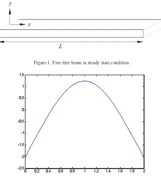
Figure 1. Free-free beam in steady state condition
Figure 3. 2ndmode shape