Degradation of Covariance Reconstruction

(1)

Degradation of Covariance Reconstruction-Based

Robust Adaptive Beamformers

Samuel D. Somasundaram

General Sonar Studies

Thales U.K. Stockport, U.K.

Email: [email protected]

Andreas Jakobsson

Dept. of Mathematical Statistics

Lund University Lund, Sweden Email: [email protected]

Abstract—We show that recent robust adaptive beamformers, based on reconstructing either the noise-plus-interference or the data covariance matrices, are sensitive to the noise-plus-interference structure and degrade in the typical case when interferer steering vector mismatch exists, often performing much worse than common diagonally loaded sample covariance matrix based approaches, even when signal-of-interest steering vector mismatch is absent.

I. INTRODUCTION

Adaptive beamforming can be used in radar and sonar applications, e.g., for source localization, power estimation, and improving detection (see, e.g., [1], [2]). Given the model

xn=sna0+nn (1)

wherexn,sn,a0, andnndenote thenth array snapshot vector,

the nth signal-of-interest (SOI) complex waveform sample, the true SOI array steering vector (ASV), and the nth noise-plus-interference (NPI) snapshot, such works are based on the forming of data-adaptive beamformers striving to pass the SOI from some assumed generic direction undistorted while attempting to minimize the influence of the noise and interfer-ence, including signals from other directions. In practice, the assumed SOI ASV is subject to various types of mismatch, e.g., due to pointing and/or array calibration errors, some of which are well modeled as an arbitrary mismatch [2], [3]. The NPI is often assumed to comprise far-field point interferers embedded in full-rank noise with a covariance matrix of the formQ=E

nnnH_n =Pd

i=1σ 2

iaia H

i +N, whereai,σ

2

i,d

andN denote theith interferer ASV, theith interferer power, the (typically unknown) number of interferers, and the full-rank noise covariance matrix. The interferer ASVs are subject to the same errors as the SOI and will therefore, likely also have an arbitrary mismatch component. Further, the interfer-ence ASVs can deviate significantly from those due to far-field point sources if, for instance, there are near-far-field sources or directional platform noises. Thus, it is beneficial for an adaptive beamformer to be insensitive to the NPI structure. The classical Capon, or minimum power distortionless response (MPDR), beamformer, whose M-dimensional filter, say w, being focused at a given direction, is constructed such that the power at the filter output is minimized, while being constrained to pass the given spatial frequency of interest undistorted, i.e.,

w= arg min

w

wHRw s.t. wH¯a= 1 (2)

where R = E

xnxH

n and ¯a denote the data covariance

matrix and the assumed known SOI ASV. The well-known Capon or MPDR solution is given by (see, e.g., [1], [2])

w= R

−1 ¯

a

¯

aH_R−1_¯_a (3)

As R is typically unknown, it is generally replaced with the sample covariance matrix (SCM) estimate

ˆ

RSCM= 1 N

N

X

n=1

xnxHn (4)

where N observations of the snapshot vector xk, for k =

1, . . . , N, are assumed available. It is well-known that the

SCM-based Capon beamformer is sensitive to SOI ASV and SCM estimation errors and, therefore, a wealth of robust adap-tive beamforming methods have been proposed (see, e.g., [1], [2]). Diagonal loading of the SCM is often used to address sensitivity issues [1], [2], [4]–[6], and recently also worst-case performance optimization-based or equivalently robust Capon beamformer (RCB) techniques [4]–[6], which assume that the SOI ASV belongs to an ellipsoidal uncertainty set and find the optimal diagonal loading that satisfies this assumption. It is worth noting, however, that the SCM-based Capon beamformer is not sensitive to the structure of the NPI, as none is assumed. Recently, there has also been interest in instead using a NPI covariance matrix reconstruction [7]. The rationale for this approach is that the minimum variance distortionless response (MVDR) beamformer, formulated using the NPI covariance matrix Qinstead ofRin (2), with solution (cf. (3))

w= Q

−1 ¯

a

¯

aH_Q−1_¯_a (5)

is less sensitive than the Capon approach to SOI ASV er-ror [1]. In passive sensing, when SOI-free samples, nn, are unavailable, a SCM estimate of Qcannot be obtained. In [7],

(2)

loaded SCM-based methods such as the RCB. Next, we briefly review some robust beamformers, including the recent iterative adaptive approach (IAA) algorithm [8], which itself is a data covariance matrix reconstruction approach, also introducing novel covariance reconstruction based beamformers. Then, in Section III, we examine the performance of the beamformers in the presence of interference ASV errors and arbitrary SOI ASV errors. Finally, we conclude the work in Section IV.

II. ROBUST BEAMFORMERS

To reduce sensitivity to SOI ASV errors and to SCM estimation errors, several robust versions of the Capon beam-former have been developed; one of the more well-known is the RCB, which constructs the beamformer as [5]

min a

aHR−1a s.t. (a−¯a)H_C−1

(a−¯a)≤1 (6)

where C is some (known) positive definite matrix describing the uncertainty ellipsoid axes. This estimator has been found to yield notable robustness to ASV and SCM errors, and has been extended in various forms. In the following, using the SCM estimate (4) in (6) to obtain an estimated SOI ASV and then using the estimates in (3) is denoted the RCB.

An alternative recent approach is to instead use a NPI co-variance matrix reconstruction with the MVDR equation (5) to form a beamformer that suppresses the SOI-free measurements as well as possible. There are several options for reconstructing

Q. In [7], SCM-based Capon estimates are exploited to form ˆ

Q. Let Θ and Θ˜ denote disjoint sets of angles denoting the region containing the SOI and the region where it is assumed not to reside, respectively. Then, the NPI covariance matrix may be reconstructed from the observed data as [7]

ˆ Capon-based spatial spectrum at angle θ. Letting θ_Θ˜ denote a vector of NΘ˜ angles that uniformly sample Θ, (7) may be˜ approximated using a summation over the ASVs formed at each of theN_Θ˜ angles, that is, as [7] associated Capon estimates, σˆ2

Capon(θ), along the main diago-nal. We denote the beamformer resulting from using the so-obtained estimate Qˆ in (5) the MVDR-Q-Capon beamformer. In [7], to further allow for SOI ASV mismatch, the SOI ASV is updated according to ˆa= ¯a+e⊥, wheree⊥ is found from

min e_⊥

(¯a+e⊥)HQˆ−1(¯a+e⊥)

s.t. ¯aHe⊥= 0, (¯a+e⊥)HQˆ(¯a+e⊥)≤a¯HQˆ¯a (9)

UsingaˆandQˆ in (5) yields the Recon-Est beamformer, which we include here for completeness.

Alternatively, one could form the beamformer using (3) with a reconstruction of the data covariance matrixR. Such a

reconstruction can be formed using Qˆ, i.e., as

ˆ

where θΘ denotes a vector of NΘ angles uniformly sampling

Θ. We remark that theK=NΘ+N_Θ˜ angles inθ contain the

angles inθΘ andθ_Θ˜. When usingRˆCapon in (3), the resulting beamformer is termed the MPDR-R-Capon beamformer. The data covariance matrixR may instead be reconstructed using the IAA-framework, i.e., as the solution obtained by iteratively solving a weighted least squares amplitude estimate for each considered spatial frequency, and then using these to form the resulting covariance matrix estimate, iterating

ˆ

until practical convergence, whereA(θ₎_∈CM×K_{contains the} K steering vectors sampling the entire space at the directions defined in θ _∈ RK×1

, PˆIAA(θ₎ _∈ RK×K

is a diagonal matrix containing the IAA power estimates, Pk, along the

diagonal, where a(θk) denotes the presumed steering vector

at direction θk, and sˆk(n) the nth complex amplitude at

directionθk [8]. At initialization, one typically setsRˆIAA=I. We will denote the MPDR-style beamformer resulting from using (3) with RˆIAA, as obtained using (11), after letting the IAA algorithm converge, MPDR-R-IAA. Comparing (10) and (11), we observe that the only difference in the MPDR-R-IAA and MPDR-R-Capon approaches is that Capon or IAA power estimates are used to reconstruct the data covariance R.

Clearly, one may also use RˆIAA to form an estimate of

Q, such that instead of exploiting the Capon spatial spectrum estimator in (7), one could exploit the IAA-spectrum estimator to reconstruct Q, yielding

ˆ

where A(θ_Θ)_{denotes the matrix of presumed ASVs for a set} of directions that uniformly sample the set of anglesΘ, which are assumed to contain the SOI, and where PˆIAA(θ_Θ) _{is a} diagonal matrix containing the associated power estimates in these directions. When usingQˆIAAin (5), we term the resulting algorithm the MVDR-Q-IAA beamformer. The MVDR-Q-IAA and MPDR-R-Capon beamformers are novel and are in-cluded as they relate the existing MVDR-Q-Capon [7] and MPDR-R-IAA (IAA) [8] approaches.

III. NUMERICALEXAMPLES

(3)

20 40 60 80 100 120 140 160 −10

0 10 20 30 40

Azimuth angle

Power (dB)

MPDR−SCM RCB−SCM MPDR−R−IAA MVDR−Q−IAA MPDR−R−Capon MVDR−Q−Capon Recon−Est IAA

20 40 60 80 100 120 140 160 −10

0 10 20 30 40

Azimuth angle

Power (dB)

90 91 36

38 40

(a) (b)

20 40 60 80 100 120 140 160 −10

0 10 20 30 40

Azimuth angle

Power (dB)

89 90 36

38 40

20 40 60 80 100 120 140 160 −10

0 10 20 30 40

Azimuth angle

Power (dB)

(c) (d)

20 40 60 80 100 120 140 160 −10

0 10 20 30 40

Azimuth angle

Power (dB)

20 40 60 80 100 120 140 160 −10

0 10 20 30 40

Azimuth angle

Power (dB)

(e) (f)

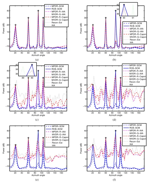
Fig. 1. ForN= 60_snapshots,σ2

0= 40dB and

¯

θ= 90◦_{and (a)}δ_θ= 0_,σ2

e,0=σ 2

e= 0, (b)δθ= 1◦,σe,20=σ 2

e = 0(c)δθ=−1.22◦,σ 2

e,0=σ 2

e= 0, (d)δ_θ=₋1.22◦_,σ2

e,0= 0.25,σ 2

e= 0, (e)δθ=−1.22◦,σ 2

e,0= 0,σ 2

e= 0.25, and (f)δθ=−1.22◦,σ 2

e,0= 0.25,σ 2

(4)

and arbitrary SOI ASV errors. We consider a simulated M = 20 element half-wavelength spaced uniform linear array, assuming that the NPI covariance has the form Q = Pd

i=1σ 2

is(θi)sH(θi) + I, where σ2i is the ith interference

power, and s(θi) = a(θi) +σeei, with ei denoting a

zero-mean complex circularly symmetric random vector with unit norm. Thus, when σe 6= 0, the interference ASV s(θi) will

be arbitrarily mismatched. Although this is often not taken into account, it should be noted that the interference ASVs will typically be subject to arbitrary mismatch in much the same way as the SOI ASV is. Furthermore, the NPI may include signals in the near-field and may not even be due to point sources. Ideally, an adaptive beamformer should be insensitive to the structure of the noise and interference. Here, we assume d = 3 interferences nominally at 21◦

, 60◦

, and

105◦

with powers of20,30, and30dB, and simulate the SOI ASV as a0 = a(¯θ+δθ) +σe,0e0, where θ¯is the assumed SOI AOA, δθ an angle mismatch,σe,0 the norm of the ASV mismatch, and e0 is defined similarly to ei. For the matrix

reconstructions, we consider a grid ofK= 180angles, equally spaced between 1◦

and180◦

. For all of the tested algorithms we examine the spatial spectra, i.e.,wHRˆSCMwfor each beam, assuming that the beams are formed at ∆ = 3◦

steps in the interval[3◦

,177◦

], so that there are 59 beam directions in total. The nominal interference angles are each on one of the K grid angles. In the following, we introduce interference AOA mismatch, where each of the interference AOAs are drawn from a uniform distribution whose limits are within ±0.5∆ of the nominal AOA, so that they may not necessarily lie on a grid point. For comparison purposes, we also evaluate the MPDR-R-IAA (IAA) algorithm at all K = 180 grid angles, terming this simply IAA. For beam direction θ, it is assumed¯ that the SOI can belong to the interval [¯θ−∆/2,θ¯+ ∆/2]◦

. This leads to values ofNΘof between 6 and 7. Tight spherical uncertainty sets were used with the RCB, whose steer-direction dependent radii were calculated using the technique outlined in [9], where a minimum value radius of 1 was imposed. For a SOI nominally atθ¯= 90◦

with powerσ2

0 = 40dB, Fig. 1(a) illustrates the spatial spectra when there are no AOA or arbi-trary errors in the SOI or interference ASVs. Fig. 1(b) shows the spectra when the SOI is simulated with δθ = 1◦ AOA

mismatch, illustrating that MPDR-R-Capon, MPDR-R-IAA, and MPDR-SCM will all undergo severe SOI cancellation, whilst MVDR-Q-IAA, MVDR-Q-Capon and Recon-Est are more robust, whereas the RCB yields the most robust estimate. The IAA algorithm does not undergo signal cancellation as the SOI AOA coincides with one of its steer directions. For the other reconstruction-based algorithms, even though the SOI AOA does not coincide with a beam steer direction, it does coincide with one of theK grid points used in the covariance matrix reconstruction. In Fig. 1(c), the spectra when the SOI is simulated withδθ=−1.22◦are illustrated, so that its AOA

no longer coincides with one of the K grid points, showing that the noise floors for MVDR-Q-Capon, Recon-Est and MPDR-R-Capon have increased significantly. The noise-floors for MVDR-Q-IAA and MPDR-R-IAA are largely unchanged, highlighting the benefits of using IAA power estimates instead of Capon ones to reconstruct the covariance matrices. The IAA algorithm does now exhibit SOI cancellation as the SOI AOA no longer coincides with one of the K grid points. The RCB exhibits the least SOI cancellation. Finally, in Figs. 1(d),

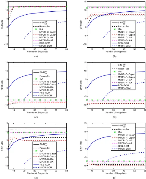
(e), and (f), we arbitrarily mismatch the SOI ASV only, the interference ASVs only, and both the SOI and interference ASVs, indicating a clear degradation of the noise floor for all of the covariance reconstruction based methods, including IAA. As can be noted from these figures, this degradation of the noise floor will affect weak targets. We proceed to examine the performance as a function of the SINR, here defined as σ2

0|wHa0|2/wHQw, where σ02 is the SOI power. Fig. 2(a) illustrates the SINR as a function of N when there is no mismatch in any of the ASVs, illustrating that the covariance matrix reconstruction approaches perform significantly better than the SCM-based RCB and MPDR estimates. In Fig. 2(b), interferer AOA mismatch is introduced and one may observe a degradation in the algorithms that attempt to reconstruct covariance matrices. The degradation is more pronounced for the Capon-based reconstructions as compared with the IAA-based ones. In Fig. 2(c), arbitrary mismatch is introduced to the interference ASVs only, which leads to an extreme degradation of the reconstruction-based algorithms. Similar results are obtained in Figs. 2(d), when AOA and arbitrary errors are introduced into the interferer ASVs only. In Fig. 2(e), AOA errors are introduced into both SOI and interference ASVs, whilst in Fig. 2(f) AOA and arbitrary errors are introduced into both the SOI and interference ASVs. These results highlight that the covariance matrix reconstruction based approaches are highly sensitive to the structure of the interference and noise, which is a significant deficiency in practice.

IV. CONCLUSIONS

The performances of algorithms based on covariance ma-trix reconstruction can degrade significantly when the noise-plus-interference is not well-modeled by the assumed covari-ance structure, for instcovari-ance when arbitrary array errors exist and/or when the interferer directions of arrival do not lie on the assumed grid. Whilst IAA-based reconstruction algorithms can be used to mitigate the effect of the latter, they are still sensitive to the former. The RCB is insensitive to such errors.

REFERENCES

[1] H. L. V. Trees,Detection, Estimation, and Modulation Theory, Part IV, Optimum Array Processing. John Wiley and Sons, Inc., 2002. [2] P. Stoica and J. Li,Robust adaptive beamforming. John Wiley & Sons,

2005.

[3] R. T. Compton, “The Effect of Random Steering Vector Errors in the Applebaum Adaptive Array,” IEEE Trans. Aerosp. Electron. Syst., vol. 18, no. 5, pp. 392–400, September 1982.

[4] S. A. Vorobyov, A. B. Gershman, and Z.-Q. Luo, “Robust Adaptive Beamforming Using Worst-Case Performance Optimization: A Solution to the Signal Mismatch Problem,”IEEE Trans. Signal Process., vol. 51, no. 2, pp. 313–324, February 2003.

[5] P. Stoica, Z. Wang, and J. Li, “Robust Capon Beamforming,”IEEE Signal Process. Lett., vol. 10, no. 6, pp. 172–175, June 2003.

[6] J. Li, P. Stoica, and Z. Wang, “On Robust Capon Beamforming and Diagonal Loading,” IEEE Trans. Signal Process., vol. 51, no. 7, pp. 1702–1715, July 2003.

[7] Y. Gu and A. Leshem, “Robust Adaptive Beamforming Based on Interfer-ence Covariance Matrix Reconstruction and Steering Vector Estimation,” IEEE Trans. Signal Process., vol. 60, no. 7, pp. 3881–3885, Jul. 2012. [8] T. Yardibi, J. Li, P. Stoica, M. Xue, and A. B. Baggeroer, “Source

Localization and Sensing: A Nonparametric Iterative Approach Based on Weighted Least Squares,”IEEE Trans. Aerosp. Electron. Syst., vol. 46, no. 1, pp. 425–443, January 2010.

(5)

10 20 30 40 50 60 −10

−5 0 5 10 15

Number of Snapshots

SINR (dB)

SINRopt

ES

Recon−Est IAA

MVDR−Q−Capon MPDR−R−Capon MVDR−Q−IAA MPDR−R−IAA RCB−SCM MPDR−SCM

10 20 30 40 50 60 −10

−5 0 5 10 15

Number of Snapshots

SINR (dB)

SINRopt

ES

Recon−Est IAA

(a) (b)

10 20 30 40 50 60 −10

−5 0 5 10 15

Number of Snapshots

SINR (dB)

SINRopt

ES

Recon−Est IAA

10 20 30 40 50 60 −10

−5 0 5 10 15

Number of Snapshots

SINR (dB)

SINRopt

ES

Recon−Est IAA

(c) (d)

10 20 30 40 50 60 −10

−5 0 5 10 15

Number of Snapshots

SINR (dB)

SINRopt

ES

Recon−Est IAA

10 20 30 40 50 60 −10

−5 0 5 10 15

Number of Snapshots

SINR (dB)

SINRopt

ES

Recon−Est IAA

(e) (f)

Fig. 2. SINR vsN_{for a 0 dB SOI, with no SOI ASV error and interferers with (a) no ASV errors, (b) AOA errors but no arbitrary error, (c) arbitrary error} (σ2

e = 0.25) but no AOA error, (d) with AOA and arbitrary errors (σ

2

e = 0.25); (e) SOI and interferers with AOA error but no arbitrary errors, (f) SOI and interferers with both AOA and arbitrary errors (σ2

e,0=σ 2