CLASSIFIER LEARNING FOR IMBALANCED DATASET
USING MODIFIED SMOTEBOOST ALGORITHM AND ITS
APPLICATION ON CREDIT SCORECARD MODELING
RIFAN KURNIA
GRADUATE SCHOOL
BOGOR AGRICULTURAL UNIVERSITY
BOGOR
STATEMENT ABOUT THESIS AND INFORMATION
SOURCES
I hereby declare that the thesis entitled Classifier Learning For Imbalanced Dataset Smoteboost Using Modified Algorithm And Its Application On Credit Scorecard Modeling is my work with the direction of the supervising committee and has not been submitted in any form to any college. Resources originating or quoted from works published and unpublished from other writers have been mentioned in the text and listed in the Bibliography at the end of this thesis.
Jakarta, September 2013
Rifan Kurnia
RINGKASAN
RIFAN KURNIA. Metode Klasifikasi untuk Data Tak Seimbang Menggunakan Algoritma SMOTEBoost Termodifikasi dan Aplikasinya pada Pemodelan Penilaian Kredit. Dibimbing oleh BAGUS SARTONO dan I MADE SUMERTAJAYA.
Pada banyak kasus riil, masalah ketidakseimbangan data sering dijumpai. Data dikatakan tidak seimbang jika ada satu atau lebih kelas yang mendominasi keseluruhan data sebagai kelas mayoritas dan kelas lainnya menjadi minoritas. Pada klasifikasi statistik, ketidakseimbangan data ada masalah yang serius. Pada banyak kasus, salah mengklasifikasikan objek dari kelas minoritas bisa berdampak lebih besar daripada salah mengklasifikasikan objek dari kelas mayoritas. Sebagai contoh pada penilaian kredit, menerima pemohon kredit yang
“buruk” akan lebih berisiko daripada menerima pemohon kredit yang “baik”. Penelitian ini akan mendiskusikan salah satu teknik hibrid antara SMOTE
dan Boosting, yang disebut dengan SMOTEBoost untuk mengatasi permasalahan ketidakseimbangan pada data. SMOTE membangkitkan sampel-sample semu berdasarkan karakterik dari objek dan k-tetangga terdekat. Pembangkitan sampel semu mempunyai prosedur yang berbeda untuk tiap variabel numerik dan kategorik. Jarak Euclid digunakan untuk variabel numerik, sementara modus dari variabel digunakan untuk variabel kategorik. “Boosting” merupakan metode umum untuk meningkatkan performa dari sebuah algoritma. Pada teorinya,
boosting dapat digunakan untuk mereduksi galat secara signifikan dari algoritma pembelajaran lemah yang hanya lebih baik dari menebak kelas secara acak.
“Adaboost” merupakan jenis boosting yang popular digunakan, yang merupakan kepanjangan dari adaptive boosting.
SMOTEBoost adalah kombinasi dari SMOTE dan algoritma boosting. Tujuan dari pengkombinasian ini adalah untuk menciptakan model yang kuat dalam mengklasifikasi data yang tak seimbang tanpa mengorbankan akurasi keseluruhan. Pohon keputusan, dengan algoritma CART, akan digunakan pada setiap iterasi boosting.
Dari hasil analisis, kombinasi dari SMOTE dan boosting terbukti dapat memberikan performa yang lebih baik secara signifikan daripada hanya menggunakan CART. Saat SMOTE meningkatkan performa dari kelas minoritas, prosedur boosting meningkatkan akurasi prediksi dari teknik klasifikasi dengan berfokus pada objek yang sulit diklasifikasi. Sebagai perbandingan, SMOTEBoost
menghasilkan pemisahan yang lebih baik antara objek “baik” dan “buruk” yang ditunjukkan dari nilai ukuran performa yang lebih tinggi (KS-Statistics, Area under ROC, and Accuracy) daripada CART. Dan juga SMOTEBoost menghasilkan nilai persentase yang stabil antara sensitivitas dan spesifitas model, inilah yang menjadi perbedaan antara SMOTEBoost dan CART. SMOTEBoost
menghasilkan performa yang bagus dalam memprediksi kelas minoritas dan juga menjaga performa kelas mayoritas tetap baik. Sementara jika hanya menggunakan
Disamping memberikan performa yang lebih baik dibandingkan hanya menggunakan CART, SMOTEBoost juga menghasilkan performa yang stabil pada berbagai tingkat keburukan. Hasil uji stabilitas menunjukkan SMOTEBoost
memberikan performa yang bagus dan stabil, walaupun tingkat keburukan diatur hingga jauh lebih rendah daripada tingkat kebaikan.
SUMMARY
RIFAN KURNIA. Classifier Learning For Imbalanced Dataset Using Modified SMOTEBoost Algorithm And Its Application On Credit Scorecard Modeling. Under supervision from BAGUS SARTONO and I MADE SUMERTAJAYA.
In many real cases, imbalanced class problem are often founded. A dataset is called imbalanced if there is one or more classes that are dominating the whole dataset as majority classes, and other classes becoming minority. In statistical classification, imbalanced class is a serious problem. This could lead the model less sensitive in classifying minority class objects. In many cases, misclassifying the minority class objects could have bigger problem than misclassifying the
majority class. For instance in credit scorecard, accepting “bad” applicant will be
much risky than rejecting “good” applicant.
This study will discuss a hybrid technique between SMOTE and Boosting, called SMOTEBoost to overcome imbalanced class issue. SMOTE generates
synthetic samples based on the objects’ characteristics and the k-nearest neighbor. Synthetic samples generation has different procedure for each numerical and categorical variable. Euclidian distance is used for numerical variable, while the
value’s mode can be simply used for categorical variable. “Boosting” is a general method for improving the performance of any learning algorithm. In theory,
boosting can be used to significantly reduce the error of any “weak” learning
algorithm that consistently generates classifiers which only a bit better than random guessing. The popular variant of boosting called “AdaBoost”, an abbreviation for adaptive boosting.
SMOTEBoost is a combination of SMOTE and boosting algorithm. The purpose of this combination is to create a powerful model in classifying imbalanced class dataset without sacrificing the overall accuracy. Decision tree, with CART algorithm, will be used in each boosting iteration.
From the analysis result, the combination of SMOTE and Boosting has proven that it gives significantly better performance than CART. While SMOTE let the classifier improves the performance on the minority class, boosting procedure improves the predictive accuracy of any classifier by focusing on difficult objects. On comparison, SMOTEBoost produce better separation between good and bad class which is represents by higher performance measures (KS-Statistics, Area under ROC, and Accuracy) than CART. It also turns out that SMOTEBoost produces stable percentage between sensitivity and specificity, and this is the difference between SMOTEBoost and CART. SMOTEBoost produces good performance in predicting minority class (bad) as well as maintaining good performance in predicting majority class (good). Meanwhile if CART used, it will only gives good performance on predicting majority class.
Besides having better performance compare to CART, SMOTEBoost also maintains stable performance across different bad rate. The stability assessment result shows SMOTEBoost gives good and stable performance, even though the bad rate is set to be significantly lower than the good rate.
© Copyright owned by IPB, 2013
Copyright Act protected by Law
Prohibited from quoting part or all of this paper without including or citing sources. Citations only for educational purposes, research, writing papers, preparing reports, writing criticism, or review a matter, and the citations do not harm the interest to IPB.
CLASSIFIER LEARNING FOR IMBALANCED DATASET
USING MODIFIED SMOTEBOOST ALGORITHM AND ITS
APPLICATION ON CREDIT SCORECARD MODELING
RIFAN KURNIA
Thesis
as one of the requirements to obtain Master of Science in Applied Statistics Program.
SEKOLAH PASCASARJANA
INSTITUT PERTANIAN BOGOR
Thesis Title : Classifier Learning For Imbalanced Dataset Smoteboost Using Modified Algorithm And Its Application On Credit Scorecard Modeling
Name : Rifan Kurnia
NRP : G152110171
Major : Applied Statistics
Approved by,
Supervising Comission
Dr. Bagus Sartono, S.Si, M.Si Supervisor
Dr. Ir. I Made Sumertajaya, M.Si Co-Supervisor
Acknowledged by,
Head of Applied Statistics Study Program
Dr. Ir. Anik Djuraidah, MS
Dean of The Graduate School of IPB
Dr. Ir. Dahrul Syah, M.Sc. Agr
ACKNOWLEDGEMENT
Developing a good research is never a one-person show. I would like to
express my gratitude to people who have supported me in this endeavour. I would
like to thank:
1. My Family, Dad, Mom, and brothers, for their unlimited support and
constant prayers.
2. Dr. Bagus Sartono and Dr. I Made Sumertajaya for their precious suggestion
and guidance.
3. All lecturer in IPB Statistics Department for the valuable knowledges during
my college time.
4. Accenture Risk Analytics Team and Citibank Decision Management Team
for helping me to enhance my knowledge in data mining and credit
scorecard theory.
5. My friends at Statistics Department for their valuable support.
I hope this thesis research would be useful in the development of credit
scorecard modeling in the future. Any constructive suggestion is highly
encouraged to develop this research further.
Jakarta, September 2013
TABLE OF CONTENT
Page Number
LIST OF TABLES ... xi
LIST OF FIGURES ... xii
LIST OF APPENDIX ... xiii
1 INTRODUCTION ... 1
Background ... 1
Objective ... 2
2 LITERATURE REVIEW ... 3
Classification ... 3
Imbalanced Class Problem ... 3
Synthetic Minority Oversampling Technique - SMOTE ... 4
Classification and Regression Tree ... 5
Boosting ... 6
SMOTEBoost ... 7
Performance Measure ... 8
3 METHODOLOGY ... 10
Data ... 10
Analysis Process ... 11
4 RESULT AND DISCUSSION ... 13
Modeling Preparation ... 13
SMOTEBoost Comparison with Plain Classifier ... 13
SMOTEBoost Stability ... 16
5 CONCLUSION AND RECOMMENDATION ... 19
BIBLIOGRAPHY ... 20
APPENDIX ... 21
LIST OF TABLES
Page Number
1 Confusion matrix……... 8
2 Performance comparison SMOTEBoost vs CART ... 14
3 Event classification comparison SMOTEBoost vs CART ... 15
4 Proportion of good/bad before and after SMOTE ... 17
5 Performance comparison between various imbalanced levels ... 17
LIST OF FIGURES
Page Number
1 Illustration of imbalanced class problem in dataset ……….... 4
2 3 Example of k-NN for xi (k=6) and Synthetic samples generation using SMOTE ………... Decision tree illustration ………...………... 5 6 4 Analysis process scheme ………..……... 11
5 SMOTEBoost vs CART comparison flow chart ………..…………... 12
6 SMOTEBoost stability assessment flow chart…………..…………... 12
7 Misclassification rate chart for each iteration ……..……….. 14
LIST OF APPENDIX
Page Number
1 Predictor Variables Description ... 24
2 Predictors Relationship Summary With The Target Variable ... 27
3 Variable Importance ... 28
4 SMOTEBoost Assessment Score Ranking ... 25
5 CART Assessment Score Ranking ... 26
7 Single CART Diagram ... 27
8 R Syntax for SMOTE ... 29
1 INTRODUCTION
Background
In statistical modeling, classification is a task of assigning objects to one of several predefined categories (Tan et al., 2006). Classification modeling is useful for categorizing and organizing information in dataset systematically, making it easier for decision makers to make a policy associated with the data.
In many real-life problems, imbalanced class issue in datasets frequently occurs. It is about the existence of one or several classes having much larger proportions than other classes. This problem can affect the model performance seriously if the plain classifiers are used. Learning algorithms that do not consider class-imbalance tend to be overwhelmed by the majority class and ignore the minority class (Liu et al., 2009).
Some traditional approaches such as Logistic Regression, Discriminant Analysis, and Decision Tree. This shows us traditional classification techniques that are common used before are not suitable in handling imbalanced-class cases, since those techniques will tend to classify objects to the majority class instead of the minority class. Therefore this problem needs more techniques development in imbalanced class classification.
Several studies have been conducted in this imbalanced class classifier development. One of them is in a credit scorecard application which is explained by Brown (2012). Brown (2012) compared some classifier techniques with various imbalanced class proportion in credit scorecard data application. The result is that Gradient Boosting/Boosted Tree techniques with AdaBoost algorithm delivered the highest performance than other techniques.
Liu et al. (2009) and He et al. (2009) introduced several techniques for imbalanced class problem classification in pre-modeling step with oversampling and undersampling concept. The simplest technique is random oversampling and random undersampling. Random oversampling generates objects from minority class randomly based on its characteristics, while random undersampling removes objects from majority class. Both of them aim to balancing the proportion between majority and minority class, so the model can perform better.
Along with the development studies in imbalanced class problem, several pre-modeling techniques were developed as well, based on oversampling and undersampling concept. For example, EasyEnsemble and BalanceCascade algorithm which are based on undersampling concept as in Liu et al.(2009), and SMOTE (Synthetic Minority Oversampling Technique) based on oversampling and undersampling concept as in Chawla et al. (2002).
2
neighbor (k-NN). It is expected to overcome the drawback of undersampling-based technique that omits the important information contained in the removed objects. By this reason, the author use SMOTE algorithm in the pre-modeling step.
This study conducted to apply the combination of SMOTE in the pre-modeling step and Boosted Tree in the modeling step for seeding with an imbalanced class dataset problem. A small simulation study was performed to examine the stability of the performance of the proposed approach. It was then followed by the implementation of the approach to a real-life dataset on discriminating bad debtor from the goods.
Objective
This study aims to :
1. Apply SMOTE (Synthetic Minority Oversampling Technique) at pre-modeling step and Boosted Tree Classifier at modeling step on the application of credit scorecard data with imbalanced class problem.
2 LITERATURE REVIEW
Classification
Classification, which is the task of assigning objects to one of several predefined categories, is a pervasive issue that encompasses many diverse applications (Tan et al., 2006). Classification modeling consists of two step, training step and validation step. In training step, data is analyzed by classifier algorithm and resulting classification rule. Then after classification rule defined, validation data is used to see model performance. If the model performance is acceptable, then this classification rule can be used to classify a new dataset.
Imbalanced Class Problem
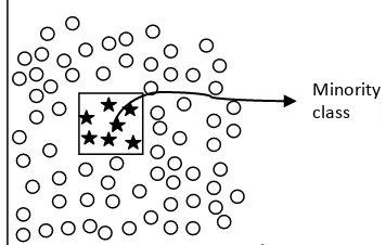
In many real cases, imbalanced class problem are often founded A dataset is called imbalanced if there is one or more classes that are dominating the whole dataset as majority classes, and other classes becoming minority. This problem is represented as in Figure 1. Objects
from the first class (notated as “o”) dominate the dataset, and in another side objects from the second class (notated as ””) has a much fewer amount in the dataset.
Some real cases could be served as examples for describing this imbalanced class problem. For example in building credit scorecard model, imbalanced problem is almost always found because the good debtors are much larger than the bad debtors. Of course this is usually happened since the bank will always analyze the debtor candidates’ profile before giving them approval. Another case of imbalanced problem often occurs in rare disease detection, for example cancer. Commonly in some regions, the cancer positives will become minority proportionally than the negatives. This case will be crucial if there are misclassifications. The same problem is often founded in direct marketing case, which companies offer their product directly to their potential customers, for example by telephone, mail, etc. Usually in every marketing campaign, the customers who are interested to buy the campaigned product are much less than they who are not interested. Modeling approach that is accommodating this imbalanced class characteristic will be much more powerful to determine the potential customers.
In statistical classification, imbalanced class is a serious problem. This could lead the model less sensitive in classifying minority class objects. In many cases, misclassifying the minority class objects could have bigger problem than misclassifying the majority class. For
instance in credit scorecard, accepting “bad” applicant will be much risky than rejecting “good”
applicant.
4
Figure 1.Illustration of imbalanced class problem in dataset
Synthetic Minority Oversampling Technique – SMOTE
While random oversampling generates the similar objects from the dataset, Chawla et al.
(2002) propose a different approach in oversampling technique for handling the imbalanced data named SMOTE (Synthetic Minority Oversampling Technique). SMOTE generates synthetic
samples based on the objects’ characteristics and the k-nearest neighbor. Synthetic samples generation has different procedure for each numerical and categorical variable. Euclidian
distance is used for numerical variable, while the value’s mode can be simply used for
categorical variable. The Euclidean distance formula is defined as follows.
, = ( − )′( − ) = ( − )2 =1
The following procedure is how to generate SMOTE sampling. 1. Numerical variable
a. Take the difference between a predictor vector and one of its k-nearest neighbors b. Multiply this difference by a random number between 0 and 1
c. Add this difference to the original value of the predictor, thus creating a synthetic sample
2. Categorical variable
a. Take majority vote between the feature vector under consideration and its k-nearest neighbors for the nominal feature value. In the case of a tie, choose at random
b. Assign that value to the new synthetic class sample.
Using this technique, the new minority class samples will be created, so the proportion between majority and minority class sample will be balance. So that it will let the classifier
5
classify the object better. The number of k-nearest neighbor is defined by the model designer, based on particular practical considerations.
Figure 2. (a) Example of k-NN for xi (k=6). (b) Synthetic samples generation using SMOTE
Classification And Regression Tree
Classification and regression tree (CART) is one of non-parametric methods that employs a binary tree and classifies a dataset into a finite number of classes. CART analysis is a form of binary recursive partitioning. The CART tree consists of several nodes. The first layer consists of a root node, while the last layer consists of leaf nodes. The root node contains the entire dataset and the other nodes contain the subset of dataset. Each parent node can split into two child nodes and each of these child nodes can be split more, forming additional children as well, as illustrated in Figure 3.
The measures developed for selecting the best split often based on the degree of purity of the child nodes. One of purity measures that common be used is information gain. For example, imagine the task of learning to classify new customers into good/bad debtor groups. Information gain represents the expected amount of information that would be needed to specify whether a new instance (debtor) should be classified good or bad. The information gain for each split is as follows.
Then, the gain can be obtained by taking the difference between the information gain from parent node and the combined information gain from child nodes.
�, =� � − �(�, )
6
Figure 3. Decision tree illustration
Boosting
Ensemble learning is designed to increase the accuracy of a single classifier by training several different classifiers and combining their decisions to output a single class variable (Galar
et al, 2011). Several ensemble techniques have been develop since this “accuracy-oriented” concept has attracted many predictive modeling experts. Some of them are bagging, random forest, and boosting.
“Boosting” is a general method for improving the performance of any learning algorithm.
In theory, boosting can be used to significantly reduce the error of any “weak” learning
algorithm that consistently generates classifiers which only a bit better than random guessing (Freund and Schapire, 1996). Various weak learner have been used for boosting study, such as RIPPER (Cohen, 1995) and decision tree (Quinlan, 1993). The popular variant of boosting called
“AdaBoost”, an abbreviation for adaptive boosting (introduced by Freund and Schapire, 1996), has been described as the best off-the-shelf classifier (Breiman, 1998).
The AdaBoost algorithm takes a training set {(x1,y1),…,(xm,ym)} as input, where x is the
predictor variable and y is the response variable. In each iteration (t = 1,2,…,T) , AdaBoost calls
specified weak learning algorithm, in this paper CART algorithm is used. The weak learner’s job
is to find a weak hypothesis ∶ � →{−1, +1}. The weight of each object, denoted with � ( ), initially are set equally, then updated iteratively and let the misclassified objects having more weight than correctly classified objects, so that the weak learner is forced to focus on the hard objects to be classified. The goodness of a weak hypothesis is measure by its error.
� = =1� �( ≠ )
� =1
I is the indicator function which is valued as 1 if the object is misclassified, or 0 if the object correctly classified by the weak learner. If the error value is greater than 0.5, then the loop will be stopped.
After the weak hypotheses obtained, AdaBoost calculate a parameter � .
� = 1− �
� Root
Node Leaf
7
Note that � 0 if � 0.5, and � gets larger as � gets smaller. The weight distribution � is next updated by multiplying it with the parameter � if the object is misclassified, while the correctly classified is stay similar from the previous. The weight distribution changes will affect the splitting rule and the variable used for the next iteration, since the misclassified instance will have more influential than other instance. In the imbalanced class problem, the minority class is more frequent incorrectly classified than the majority class. In case of tree model used, the model will learn more the minority class instances than the previous step, to find the appropriate splitting rule using information gain calculation. As the model can learn better the minority class, the performance of the model will improved as well.
Since this paper will only focus on the binary class classification ({-1, +1}), the final their weights. Although boosting can reduce variance and bias, but this is not completely true if it is applied in imbalanced class dataset. Boosting treats two misclassification types (False
Positives and False Negatives) equally. Whereas in this problem, the focus is to repair the “False Negative” into “True Positive”. Therefore, a method that can improve the model performance of
imbalanced class proportion between the majority and minority class is really needed.
Applying SMOTE together with boosting will create a model that can classify minority class better and provide a broader decision related to its minority class. This method first introduced by Chawla et al. (2003) which combine his SMOTE with Freund’s Boosting. This study will try to make a little modification in SMOTEBoost algorithm by Chawla et al. (2003), which applied SMOTE in each of the boosting iteration. The SMOTE procedure will only applied in the beginning before the boosting iteration work. The reason is, in practice it is too
risky to generate many synthetic samples, as the original object’s characteristics will be sunk by
8
Input: Sequence of m sampling units {(x1,y1),…,(xm,ym)} where xi X, yi Y = {-1,+1}
Weak learning algorithm WeakLearn Integer T specifying number of iterations
Initialize �1( ) = 1/ for all i.
Modify weight distribution �1 by creating N synthetic samples using SMOTE algorithm.
Do for t= 1,2,…,T:
1. Train WeakLearn using weight distribution � ( ). 2. Get weak hypothesis ∶ � →{−1, +1}
Where is a normalization constant (chosen so that the next iteration of weight distribution, �+1, will be amounted to 100% in total).
Output the final hypothesis (for binary dependent variable):
= sign �
=1
Note that because of � < 0.5, then � will be always greater than 1. Thus, the weights of misclassified objects are increased in every single iteration.
Performance Measure
In general, classification model performance can be measured by confusion matrix as illustrated in Table 1. In credit scorecard, bad objects are the focus of the model building, so bads will be flagged as positive and goods will flagged as negative. TP is the number of the correctly classified positive objects, FP is the number of the misclassified negative objects, TN is the number of the correctly classified negative objects, and FN is the number of the misclassified positive objects.
Table 1. Confusion matrix
9
Accuracy rate is one of the performance measures to identify how the model can predict each class correctly.
� = ( �+ �)
( �+��+��+ �)
Another performance measure that is commonly used is AUC (Area Under ROC Curve). The curve is built with plotting the Sensitivity (%TP) and Specificity (%TN). For both Accuracy and AUC, the bigger the value, the better the model is.
= % �= �
�+��
= % � = �
�+��
3 METHODOLOGY
Data
This study used a secondary dataset from the UCI Knowledge Discovery in Databases (http://kdd.ics.uci.edu/), that containing data of 1000 customers from a multinational bank
company. The dependent variable is creditors’ credit score, which is good or bad, and the predictor variables are :
1. Status of existing checking account 2. Duration in month
8. Installment rate in percentage of disposable income 9. Personal status and sex
10.Other debtors / guarantors 11.Present residence since 12.Property ownership 13.Age in years
14.Other installment plans 15.Current housing status
16.Number of existing credits at this bank 17.Job
18.Number of people being liable to provide maintenance for 19.Telephone
20.Foreign worker
11
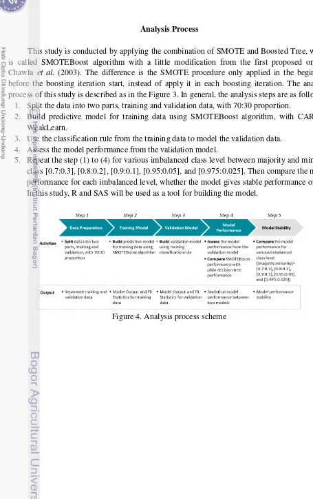
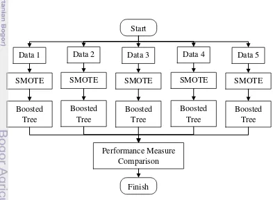
Analysis Process
This study is conducted by applying the combination of SMOTE and Boosted Tree, which is called SMOTEBoost algorithm with a little modification from the first proposed one by Chawla et al. (2003). The difference is the SMOTE procedure only applied in the beginning before the boosting iteration start, instead of apply it in each boosting iteration. The analysis process of this study is described as in the Figure 3. In general, the analysis steps are as follows.
1. Split the data into two parts, training and validation data, with 70:30 proportion.
2. Build predictive model for training data using SMOTEBoost algorithm, with CART as WeakLearn.
3. Use the classification rule from the training data to model the validation data. 4. Assess the model performance from the validation model.
5. Repeat the step (1) to (4) for various imbalanced class level between majority and minority class [0.7:0.3], [0.8:0.2], [0.9:0.1], [0.95:0.05], and [0.975:0.025]. Then compare the model performance for each imbalanced level, whether the model gives stable performance or not. In this study, R and SAS will be used as a tool for building the model.
12
Figure 5. SMOTEBoost vs CART comparison flow chart
4 RESULT AND DISCUSSION
Modeling Preparation
Before running SMOTEBoost and CART model to be compared, some parameters need to be tuned first. For CART, information gain/entropy criterion is used to train predictors as explained in previous section. One of the major problems in tree-based model is overfitting, and to prevent this problem the tree should be pruned. To perform tree pruning, the maximum depth of the tree is set to 10 nodes. This number also aligned to the parsimony principle and the industrial benchmark, which the model must be having 10 nodes at most. Besides that, the minimum number of training observations in each leaf is constrained to 10, so each node will only train variable if there are at least 10 observations in a leaf.
For SMOTEBoost, the procedure is divided into two step, firstly the minority class is oversampled by SMOTE, then the whole data are modeled by Boosted Tree algorithm. In this research, the number of nearest neighbor for SMOTE used is 5 observations. The proportion of minority class after oversampling is specified to 40% of the whole data. In Boosted Tree modeling step, the number of iteration performed is 50 iterations. The tree parameters used in Boosted Tree step is similar with CART for the purposes of comparison, with the maximum depth of tree is set to 10 nodes as well.
The synthetic samples created from the SMOTE are only used for the purposes of modeling. With SMOTE, the model enables to learn more from the minority class. To assess the performance, the synthetic samples are needed to be removed first after modeling step, which means the performance only measured from the original data.
SMOTEBoost Comparison With Plain Classifier
14
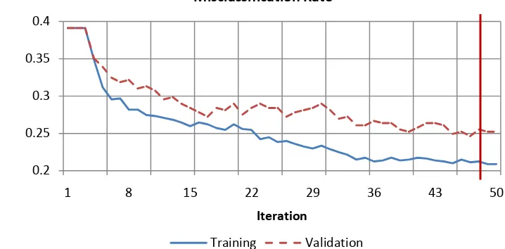
Figure 7. Misclassification rate chart for each iteration
For SMOTEBoost, after oversampling the minority with SMOTE procedure, boosting procedure is applied using CART as the base learner. As depicted on Figure 7, the boosting loop is stopped after 49 iterations. From the figure above, boosting procedure enable weak classifier to perform self-repaired as the misclassification rate trend goes down along with the looping.
Table 2. Performance comparison SMOTEBoost vs CART
Parameter
Training Validation
KS-Statistics Area Under
ROC Accuracy KS-Statistics
Area Under
ROC Accuracy
CART 47% 78% 78% 39% 74% 76%
SMOTEBoost 54% 84% 79% 46% 78% 76%
From Table 2, all of the performance parameter shows that SMOTEBoost algorithm classify much better than CART. The KS-Statistics shows the different separation power between two techniques. Both of the two techniques are in acceptable industrial benchmark for KS-Statistics, between 20% and 70%. In the training and validation sample, the KS of SMOTEBoost is 7% better than CART. This indicates that SMOTEBoost can separate good and bad class significantly better than CART. The same thing also showed by area under ROC curve (AUROC), and accuracy results, that SMOTEBoost gives significant better performance than CART. SMOTEBoost gives stronger discrimination power than CART in terms of AUROC, while maintain the good accuracy for both training and validation sample. The different performance between training and validation data are possibly due to the relatively small size of data (1000 observations). This problem is not a big problem in the pilot model development, since the data size will grow bigger in the future development.
15
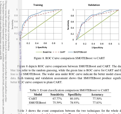
Figure 8. ROC Curve comparison SMOTEBoost vs CART
Figure 8 depicts ROC curve comparison between SMOTEBoost and CART. The diagonal blue line refer to the random guessing, while the green line is ROC curve for CART and the red line is for SMOTEBoost. The wider area under ROC curve indicate the better model classify the data. Both training and validation assessment shows that SMOTEBoost produce significantly better ROC curve compare to plain CART.
Table 3. Event classification comparison SMOTEBoost vs CART
Model Sensitivity Specificity Accuracy
CART 67.77% 80.10% 77.50%
SMOTEBoost 75.59% 78.93% 77.83%
Table 3 shows the event comparison between the two techniques for the whole dataset
(consolidated training and validation sample). The goods are denoted as “negative”, while the bads are denoted as “positive” since the predicting the bads correctly are more critical in credit
scoring development. In some literature, the percentage of true positive is called as sensitivity, while the percentage of true negative is called as specificity. In the the previous section it is already known that SMOTE increase the bad proportion from the whole data and let the classifier train the minority class more. It turns out that SMOTEBoost produces stable percentage between sensitivity and specificity, and this is the difference between SMOTEBoost and CART. SMOTEBoost produces good performance in predicting minority class (bad) as well as maintaining good performance in predicting majority class (good). Meanwhile if CART used, it will only gives good performance on predicting majority class. From the correct classification rate, it is also indicated that SMOTEBoost gives higher percentage than CART.
16
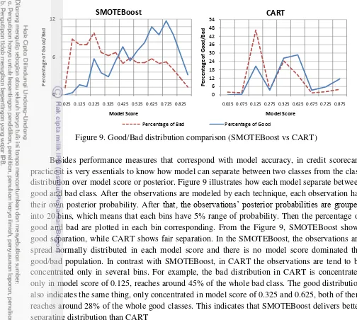
Figure 9. Good/Bad distribution comparison (SMOTEBoost vs CART)
Besides performance measures that correspond with model accuracy, in credit scorecard practice it is very essentials to know how model can separate between two classes from the class distribution over model score or posterior. Figure 9 illustrates how each model separate between good and bad class. After the observations are modeled by each technique, each observation has their own posterior probability. After that, the observations’ posterior probabilities are grouped into 20 bins, which means that each bins have 5% range of probability. Then the percentage of good and bad are plotted in each bin corresponding. From the Figure 9, SMOTEBoost shows good separation, while CART shows fair separation. In the SMOTEBoost, the observations are spread normally distributed in each model score and there is no model score dominated the good/bad population. In contrast with SMOTEBoost, in CART the observations are tend to be concentrated only in several bins. For example, the bad distribution in CART is concentrated only in model score of 0.125, reaches around 45% of the whole bad class. The good distribution also indicates the same thing, only concentrated in model score of 0.325 and 0.625, both of them reaches around 28% of the whole good classes. This indicates that SMOTEBoost delivers better separating distribution than CART
SMOTEBoost Stability
Besides compare the performance between SMOTEBoost and plain CART performance, this study also aim to assess the performance stability of the SMOTEBoost algorithm. There are five good/bad proportion that will be assess in this study, [0.7:0.3], [0.8:0.2], [0.9:0.1], [0.95:0.05], and [0.975:0.025]. In practice, the greater good/bad difference will produce worse performance if using plain classifier.
0 6 12
0.025 0.125 0.225 0.325 0.425 0.525 0.625 0.725 0.825
P
0.025 0.075 0.125 0.275 0.325 0.625 0.675 0.725 0.875
17
Table 4. Proportion of good/bad before and after SMOTE
Data Good/Bad Proportion Before SMOTE After SMOTE
Data 1 0.7:0.3
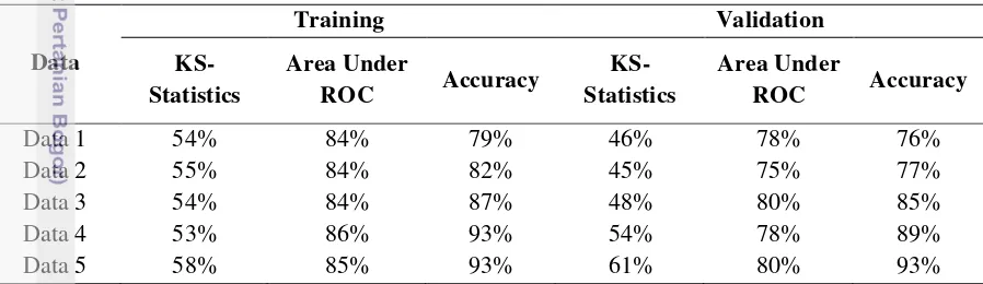
Table 4 shows the proportion between good and bad, before and after applying SMOTE to the dataset. With various proportion of good and bad in each data, SMOTE procedure oversampling the bad to the same proportion which is 40% of the whole class in each data. In general, the purpose of applying SMOTE to dataset is to balance the proportion of the class. After applying the SMOTE, the SMOTEBoost algorithm takes role to model the data. The same boosting parameters with the previous subsection are used for each data to test the stability.
Table 5. Performance comparison between various imbalanced levels
18
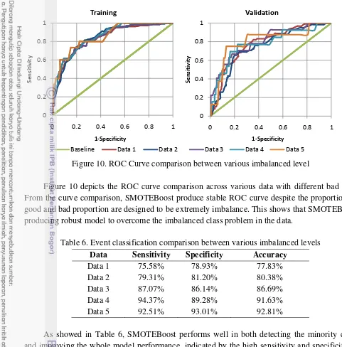
Figure 10. ROC Curve comparison between various imbalanced level
Figure 10 depicts the ROC curve comparison across various data with different bad rate. From the curve comparison, SMOTEBoost produce stable ROC curve despite the proportion of good and bad proportion are designed to be extremely imbalance. This shows that SMOTEBoost producing robust model to overcome the imbalanced class problem in the data.
Table 6. Event classification comparison between various imbalanced levels
Data Sensitivity Specificity Accuracy
Data 1 75.58% 78.93% 77.83% and improving the whole model performance, indicated by the high sensitivity and specificity in each data. Besides that, the sensitivity and specificity values in each data also produce stable percentage. Although the data is set to be extremely imbalanced, SMOTEBoost keep maintains high sensitivity and specificity. In contrast with the plain classifier, SMOTEBoost performance is getting better as the class proportion getting more imbalanced. This possibly due to the small characteristics variant in bad class and SMOTE generates synthetic samples many times over until the bad rate reach 40 percent of the whole data. This will lead the classifier learn the nearly same characteristics over and over, so the classifier will classify them correctly. Overall, it shows that SMOTEBoost is a good solution to handle extreme imbalanced class data.
CONCLUSION AND RECOMMENDATION
In many practical cases, imbalanced class problem is often encountered, making plain classification techniques difficult to produce bad and unstable performance, even become overfitting in some case. In case of imbalanced class problem, the combination of SMOTE and Boosting has proven that it gives significantly better performance than CART. While SMOTE let the classifier improves the performance on the minority class, boosting procedure improves the predictive accuracy of any classifier by focusing on difficult objects. On comparison, SMOTEBoost produce better separation between good and bad class which is represents by higher KS-Statistics than CART. Besides having better performance compare to CART, SMOTEBoost also maintains stable performance across different bad rate. The stability assessment result shows SMOTEBoost gives good and stable performance, even though the bad rate is set to be significantly lower than the good rate
BIBLIOGRAPHY
Brown, I. 2012. An experimental comparison of classification techniques for imbalanced credit scoring data sets using SAS® Enterprise Miner. SAS Global Forum 129.
Bastos, J. 2008. Credit Scoring with Boosted Decision Trees. Munich Personal RePec Archive. Breiman, L. 1998. Arcing Classifiers. The Annals of Statistics: 801:849.
Chawla, V.N., Bowyer, K.W., Hall, L.O., and Kegelmeyer, W.P. 2002. SMOTE: Synthetic Minority Over-Sampling Technique. Journal of Artificial Intelligence Research 16: 321-357. Chawla, V.N., Lazarevic, A., Hall, L.O., and Bowyer, K.W. 2003. SMOTEBoost: Improving
Prediction of the Minority Class in Boosting. Journal of KDD 107-119.
Freund, Y. and Schapire, R.E. 1999.A Short Introduction to Boosting. Journal of Japanese Society for Artificial Intelligence: 771-780.
Galar, M., Fernandez, A., Barrenechea, E., Bustince, H., and Herrera, F. 2011. A Review on Ensembles for the Class Imbalance Problem: Bagging-, Boosting-, and Hybrid-Based Approaches. IEEE Transactions on Systems 42: 463-484.
Han, J. and Kamber, M. 2006. Data Mining: Concepts and Technique 2nd Edition. San Fransisco: Morgan Kaufmann Publishers.
Hastie, T., Tibshirani, R., and Friedman, J. 2008. The Elements of Statistical Learning: Data Mining, Inference, and Prediction. New York: Springer.
He, H. and Garcia, E.A. 2009. Learning from Imbalanced Data. IEEE Transaction on Knowledge and Data Engineering 21: 1263-1284.
Liu, X.Y., Wu, J., and Zhou, Z.H. 2009. Exploratory Undersampling for Class-Imbalance Learning. IEEE Transaction on System: 965-969.
Sartono, B. and Syafitri, U.D. 2010. Ensemble Tree : An Alternative toward Simple Classification and Regression Tree. Forum Statistika dan Komputasi 16: 1-7.
Siddiqi, N. 2006. Credit Risk Scorecards: Developing and Implementing Intelligent Credit Scoring. NewJersey: John Wiley & Sons.
22
Appendix 1. Predictor Variables Description
1. Status of existing checking account (CA): (ordinal) a. CA < 0 DM
b. 0 ≤ CA < 200 DM c. CA ≥ 200 DM d. no checking account
2. Duration in month: (ratio)
3. Credit history: (nominal)
a. no credits taken/all credits paid back duly b. all credits at this bank paid back duly c. existing credits paid back duly till now d. delay in paying off in the past
e. critical account/other credits existing (not at this bank)
4. Purpose: (nominal)
6. Savings account/bonds (SA): (ordinal) a. SA < 100 DM
b. 100 ≤ SA < 500 DM c. 500 ≤ SA < 1000 DM d. SA ≥ 1000 DM
23
7. Present employment since (PE): (ordinal) a. unemployed
b. PE < 1 year c. 1 ≤ PE < 4 years d. 4 ≤ PE < 7 years e. PE ≥ 7 years
8. Installment rate in percentage of disposable income: (ratio)
9. Personal status and sex: (nominal) a. male and divorced/separated
b. female and divorced/separated/married c. male and single
d. male and married/widowed e. female and single
10.Other debtors / guarantors: (nominal) a. none
b. co-applicant c. guarantor
11.Present residence since: (ratio)
12.Property: (nominal) a. real estate
b. building society savings agreement/life insurance c. if car or other
d. unknown / no property
13.Age in years: (ratio)
24
16.Number of existing credits at this bank: (ratio)
17.Job: (ordinal)
a. unemployed/ unskilled - non-resident b. unskilled - resident
c. skilled employee / official
d. management/ self-employed/highly qualified employee/ officer
18.Number of people being liable to provide maintenance for: (ratio)
19.Telephone: (nominal) a. none
b. yes, registered under the customers name
20.Foreign worker: (nominal) a. yes
25
Appendix 2. Predictors Relationship Summary With The Target Variable
No. Predictors Relationship
1. Status of existing checking account
The lower amount of checking account, the riskier
2. Duration in month The longer duration, the riskier
3. Credit history Bad credit history will increase the risk of being default
4. Purpose The more expensive credit purpose, the riskier
5. Credit amount The higher credit amount, the riskier
6. Savings account/bonds The lower amount of saving account, the riskier
7. Present employment since The longer employment length, the less risky
8. Installment rate in percentage of disposable income
The higher installment rate, the riskier
9. Personal status and sex Single (having no dependant) are deemed to be less risky
10. Other debtors / guarantors Creditor with other guarantors are deemed to be less risky
11. Present residence since The longer residence period, the less risky
12. Property Creditors that have no property are deemed to be riskier
13. Age in years Young and old people are deemed to be riskier than middle-aged people
14. Other installment plans Creditors with other installment plan are deemed to be riskier
15. Housing Creditors that owned his house are deemed to be less risky
16. Number of existing credits at this bank
The more existing credit, the riskier
17. Job The higher job position, the less risky
18. Number of people being liable to provide maintenance for
The more dependants, the riskier
19. Telephone Creditors that registered their telephone number are easier to be contacted, and deemed to be less risky
27
Appendix 4. SMOTEBoost Assessment Score Ranking
Percentile % Response Cumulative Response
Mean Posterior Probability
5 95.122 95.122 0.827
10 97.500 96.296 0.754
15 82.500 91.736 0.706
20 65.000 85.093 0.655
25 78.049 83.663 0.608
30 60.000 79.752 0.559
35 50.000 75.532 0.514
40 37.500 70.808 0.470
45 53.659 68.871 0.421
50 35.000 65.509 0.379
55 20.000 61.400 0.342
60 22.500 58.178 0.299
65 17.073 54.962 0.263
70 35.000 53.546 0.231
75 10.000 50.662 0.207
80 5.000 47.826 0.180
85 4.878 45.256 0.146
90 10.000 43.310 0.115
95 2.500 41.177 0.090
28
Appendix 5. CART Assessment Score Ranking
Percentile % Response Cumulative Response
Mean Posterior Probablility
5 72.381 72.381 0.724
10 63.591 67.986 0.636
15 63.194 66.389 0.632
20 63.194 65.590 0.632
25 63.194 65.111 0.632
30 41.620 61.196 0.416
35 35.227 57.486 0.352
40 33.026 54.429 0.330
45 21.957 50.821 0.220
50 14.799 47.219 0.148
55 13.231 44.129 0.132
60 13.231 41.554 0.132
65 13.231 39.375 0.132
70 13.231 37.508 0.132
75 13.231 35.889 0.132
80 13.231 34.473 0.132
85 13.231 33.224 0.132
90 13.231 32.113 0.132
95 13.231 31.119 0.132
29
Appendix 6. Single CART Diagram
31
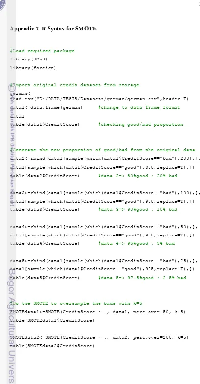
Appendix 7. R Syntax for SMOTE
#Load required package
library(DMwR)
library(foreign)
#Import original credit dataset from storage
german<-read.csv("D:/DATA/TESIS/Datasets/german/german.csv",header=T)
data1<-data.frame(german) #change to data frame format
data1
table(data1$CreditScore) #checking good/bad proportion
#Generate the new proportion of good/bad from the original data
data2<-rbind(data1[sample(which(data1$CreditScore=="bad"),200),],
data1[sample(which(data1$CreditScore=="good"),800,replace=T),])
table(data2$CreditScore) #data 2-> 80%good : 20% bad
data3<-rbind(data1[sample(which(data1$CreditScore=="bad"),100),],
data1[sample(which(data1$CreditScore=="good"),900,replace=T),])
table(data3$CreditScore) #data 3-> 90%good : 10% bad
data4<-rbind(data1[sample(which(data1$CreditScore=="bad"),50),],
data1[sample(which(data1$CreditScore=="good"),950,replace=T),])
table(data4$CreditScore) #data 4-> 95%good : 5% bad
data5<-rbind(data1[sample(which(data1$CreditScore=="bad"),25),],
data1[sample(which(data1$CreditScore=="good"),975,replace=T),])
table(data5$CreditScore) #data 5-> 97.5%good : 2.5% bad
#Do the SMOTE to oversample the bads with k=5
SMOTEdata1<-SMOTE(CreditScore ~ ., data1, perc.over=50, k=5)
table(SMOTEdata1$CreditScore)
SMOTEdata2<-SMOTE(CreditScore ~ ., data2, perc.over=200, k=5)
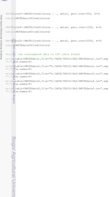
32
SMOTEdata3<-SMOTE(CreditScore ~ ., data3, perc.over=500, k=5)
table(SMOTEdata3$CreditScore)
SMOTEdata4<-SMOTE(CreditScore ~ ., data4, perc.over=1200, k=5)
table(SMOTEdata4$CreditScore)
SMOTEdata5<-SMOTE(CreditScore ~ ., data5, perc.over=2500, k=5)
table(SMOTEdata5$CreditScore)
#Export the oversampled data to CSV table format
write.table(SMOTEdata1,file="D:/DATA/TESIS/SAS/SMOTEdata1.csv",sep =",",row.names=F)
write.table(SMOTEdata2,file="D:/DATA/TESIS/SAS/SMOTEdata2.csv",sep =",",row.names=F)
write.table(SMOTEdata3,file="D:/DATA/TESIS/SAS/SMOTEdata3.csv",sep =",",row.names=F)
write.table(SMOTEdata4,file="D:/DATA/TESIS/SAS/SMOTEdata4.csv",sep =",",row.names=F)
33
Appendix 8. Proportion of Good/Bad Before and After SMOTE
Before SMOTE
70% 30%
Data 1
80% 20%
Data 2
90%
10% Data 3
95%
5% Data 4
97.50%
2.50% Data 5
%Good
%Bad
60% 40%
After SMOTE
%Good
%Bad
34
BIOGRAPHY
The author was born in Jakarta, December 24th 1989 as the first son from Ir. Rismon Nazaruddin and Dra. Deswati Noor.
In 2007, the author graduated from SMAN 12 Jakarta and continued his study to Gadjah Mada University majoring in Statistics. The author gained his Bachelor degree in 2011 and continued his study to Bogor Agricultural University majoring in Applied Statistics at the same year.