Spatial Regression Approach in Determining Factors Affecting Percentage of Human Trafficking Victims inWest Java.

SPATIAL REGRESSION APPROACH IN DETERMINING FACTORS

AFFECTING PERCENTAGE OF HUMAN TRAFFICKING VICTIMS

IN WEST JAVA

DANIA SIREGAR

DEPARTMENT OF STATISTICS

FACULTY OF MATHEMATICS AND NATURAL SCIENCES

BOGOR AGRICULTURAL UNIVERSITY

SUMMARY

DANIA SIREGAR.

Spatial Regression Approach in Determining Factors Affecting

Percentage of Human Trafficking Victims in West Java. Supervised by

ASEP SAEFUDDIN and ANANG KURNIA.

The spatial dimension plays a key role in many social phenomenons such as poverty, pollution, disease, crime and others. Social phenomenon in certain areas is influenced by the social phenomenon in other locations.

One of the interesting social phenomenons that will

be studied in this research is human trafficking in West Java. The aims of this study are

to identify the spatial effects on percentage of human trafficking victims, and to determine

the factors which affected percentage of human trafficking victims in West Java in 2010.

The existence of spatial relationship information between district/municipality led to need

to accommodate the spatial

variability in the model, so that the model used were spatial

regression models. Based on the analysis, spatial effect influential significantly the percentage

of human trafficking victims. The hotspot for human trafficking victims were Cimahi

Municipality, Bandung Municipality and Bandung District. The best model to accommodate

spatial effect in this study

was General Spatial Model (GSM)

with AIC-value=-361.46

and

R

2a=71.34%.

Based on

GSM

obtained the

indepen-dent variables or factors

which

significantly affected percentage of human trafficking victims in West Java in 2010

for

α=0.05

as follows: the average of population with divorce status, the average of population

with local

migrant status, and the

average of

population with maximum education in Junior High School.

SPATIAL REGRESSION APPROACH IN DETERMINING FACTORS

AFFECTING PERCENTAGE OF HUMAN TRAFFICKING VICTIMS

IN WEST JAVA

DANIA SIREGAR

Minithesis

as one of requirements to obtain

Bachelor's Degree of Statistics (with honors)

at Department of Statistics

DEPARTMENT OF STATISTICS

FACULTY OF MATHEMATICS AND NATURAL SCIENCES

BOGOR AGRICULTURAL UNIVERSITY

Title of Minithesis :

Spatial Regression Approach in Determining Factors Affecting

Percentage of Human Trafficking Victims in West Java.

Name : Dania Siregar

NIM : G14080015

Approved

Advisor I, Advisor II,

Prof. Dr. Ir. Asep Saefuddin, M.Sc Dr. Anang Kurnia NIP. 195703161981031004 NIP. 197308241997021001

Known

Head of Department of Statistics Faculty of Mathematics and Natural Sciences

Bogor Agricultural University

Dr. Ir. Hari Wijayanto, M.Si. NIP. 196504211990021001

ACKNOWLEDGEMENTS

Alhamdulillah, In the name of Allah The Beneficent, The Merciful praise be to Allah The Lord of The World. Blessing and salutations be upon the most honorable Muhammad saw. as prophet and messenger, his family and disciples who follow him in goodness till the day of judgment.

The paper is entitled "Spatial

Regression

Approach

in

Determining

Factors Affecting

Percentage of Human Trafficking Victims in West Java". It would not have been possible to

complete this paper without the assistance of several individuals. The author would like to thank profusely to all those who have helped, among others:

1. Prof. Dr. Ir. Asep Saefuddin, M.Sc. and Dr. Anang Kurnia, as advisory committee have provided guidance, direction, and feedback during the writing of this paper.

2. Dr. Ir. Hari Wijayanto, M.Si. and all teaching staf of Department of Statistics who have provided knowledge for author carried out study in Bogor Agricultural University.

3. The entire administrative staff and employees of Department of Statistics who always ready to assisted the author in completing various needs related to the completion of this paper. 4. Mother and father who always give love, affection and trust to the author since childhood till

now.

5. Rona Karunia Siregar, Nadia Itona Siregar, and M. Ihsan Siregar who have provided the motivation to the author in order to give best.

6. Dr. Ahmad as counselor at Al Iffah Boarding School who has provided much insight about the meaning and purpose of life.

7. Sekar Sari Utami Wiyaja, her help in scientific discussion regarding spatial regression. 8. All friends in Department of Statistics.

9. All friends in Student’s Advisory Assembly of Bogor Agricultural University (MPM KM IPB) who taught the author the meaning of brotherhood and team work.

10. All friends in Student’s Parliament of Bogor Agricultural University (DPM KM IPB) who taught the author the meaning of caring and affection to each other.

11. Ana Widiyawati, Arni Nurwida, Hilda Rafika Wati, Intan Apriliani, Miftachul Jannah, Yulia Devi Anggorosasi, Baehaki Fajri Ibnu Abbas and M. Tegar Kusmahidayat Konenda as friends who always complement each other and give encouragement to complete the mandate of the organization and the mandate of the academic with balanced.

12. All those who have provided support, prayer and motivation in completion this paper. Hopefully all the kindness rewarded by Allah swt. and this paper can be useful for all those who read it.

Bogor, January 2013

CURRICULUM VITAE

The author

named Dania

Siregar

and was born in Kalianda

on

February 27, 1991, a

daughter of couple Pandeangan Siregar, S.Pd.SD and Mely Maryati, S.Pd.SD. The author

is second daughter of four children.

In 2002 the author completed her primary school education at SDN 2 Kalianda. The

author

continued her studies

at

SMPN 1 Kalianda

and graduated

in 2005.

In 2008

the

author graduated from SMAN 1 Kalianda and

in the same year passed the selection into

the Bogor Agricultural University through the Invitation Selection of

Bogor Agricultural

University. The author chose

mayor

Statistics,

Faculty of Mathematics

and Natural

Sciences with a minor in Consumer Sciences.

TABLE OF CONTENTS

Page

LIST OF TABLES ... viii

LIST OF FIGURES ... viii

LIST OF APPENDIXES ... viii

INTRODUCTION ... 1

Background ... 1

Objective ... 1

LITERATURE REVIEW ... 1

Multiple Regression Analysis ... 1

Spatial Regression Analysis ... 2

Spatial Effect Test ... 2

Spatial Modeling ... 4

Spatial Weighting Matrix ... 4

Best Model Selection ... 5

Spatial Analysis in Human Trafficking ... 5

METHODOLOGY... 6

Data ... 6

Methods ... 6

RESULTS AND DISCUSSION ... 6

Exploring Data ... 6

Multiple Regression Analysis ... 8

Testing for Spatial Effects ... 9

Spatial Autoregressive Model (SAR) ... 10

General Spatial Model (GSM) ... 10

The Factors which Affected Percentage of Human Trafficking Victims in West Java ... 11

CONCLUSIONS AND RECOMMENDATION ... 11

Conclusions ... 11

Recommendation ... 11

REFERENCES ... 11

LIST OF TABLES

Page

1.

Distribution of frequency based on percentage interval

of human trafficking victims in West Java... 8

2.

The results of spatial dependence ... 9

3. The parameters estimation for SAR ... 10

4. The parameters estimation for GSM ... 10

5. The indicators of goodness model ... 11

LIST OF FIGURES

Page 1. Moran’s scatter plot ... 2

2. Spatial weighting illustration. ... 5

3. Diagram percentage of human trafficking victims in West Java in 2010. ... 7

4.

The thematic map of percentage interval of human trafficking victims in West Java

7 5. Normality plot for multiple regression. ... 8

6. Scatter diagram between residual and fitted value of multiple regression ... 9

7. Moran’s scatter plot ... 9

LIST OF APPENDIXES

Page 1. The independent variables ... 14

2. Descriptive statistics of the independent variables ... 15

3. Fitting linear line pattern for the variables no-multicolinearity ... 16

4. Normality plot for SAR model ... 17

5. Scatter plot between residual and fitted value for SAR model ... 17

6. Normality plot for GSM ... 17

7. Scatter Plot between residual and fitted value for GSM ... 17

1

INTRODUCTION

Background

The spatial dimension plays a key role in many social phenomenons such as poverty, pollution, disease, crime and others. Social phenomenon in certain areas is influenced by the social phenomenon in other locations as stated in the first law of geography advanced by W Tobbler cited by Anselin (1988), it is stated that everything is related to everything else, but near thing are more related than distant one. Spatial effects are relatively common happened between one region to another. Based on LeSage (1998), two problems arise when sample data has a location component: 1) spatial dependence exists between the observations and 2) spatial heterogenity occurs in the relationships which are modeling. The existence of spatial relations in dependent variable will cause estimates to be inaccurate because the assumption of randomness error is violated. To solve above problems, required a regression model that incorporates the spatial relationship between regions into the model. The existence of spatial relationship information between regions led to need to accommodate the spatial variability in the model, so that the model used is spatial regression models.

One of the interesting social phenomenons to be studied in this research is human trafficking. Human trafficking for forced labor or sexual exploitation is believed to be one of the fastest growing areas of crime. It becomes the second largest source of illegal income worldwide after drug trafficking. Combating human trafficking, or the use of force, fraud or coercion to transport persons across international borders or within countries to exploit them for labor or sex, become important priority for many goverments around the world (Belser 2005 ; Laczko 2005, referenced in Goździak and Bump 2008). Information of spatial relations that have been occurred in this case is assumed based on Sanders (2007) that the spatial interactions can be also expressed as an influence of a location on another, without being explicitly embodied in the form of a measurable exchange or flow, like life experience, trafficking trajectories or local customs.

Based on International Organization for Migration (US) (2011) in trafficking case data, Indonesia become top ten countries of destination where victims were trafficked in

2011. Beside that based on data from the Criminal Investigation Police Headquarters of the Republic of Indonesia Agency (ID), in the period 2005-2009, West Java was on the top of trafficking cases, followed by West Kalimantan, East Java, Central Java and West Nusa Tenggara. Coordinator Minister for People's Welfare in 2009, Agung Laksono, said the high incidence of human trafficking occured because human trafficking had syndicates and huge resource. In addition, the perpetrators often move transportation routes which was lack of supervision. Besides that, human trafficking was closely associated with high rates of poverty and unemployment, low level of education, gender discrimination, and early marriage and divorce (Jabar … 2009). This is the background why the author took the human trafficking cases in West Java to be analyzed using spatial regression models. The author hoped that the information from this research could help decision-makers to craft effective policies.

Objective

The aims of this study are to identify the spatial effects on percentage of human trafficking victims, and to determine the factors which affected percentage of human trafficking victims in West Java in 2010 using spatial regression model.

LITERATURE REVIEW

Multiple Regression Analysis

Multiple regression analysis is an analysis to evaluate the relationship between response variables and several explanatory variables. General multiple regression model, as follows:

with is the respond variable vector (N 1),

is the matrix of explanatory variables (N k), is the vector of regression coefficients (k 1), is the vector error no- autocorrelation (N 1), and N is the number of observations. Regression parameters expected by Least Squares Method. Regression parameter estimators:

̂

3

There are four quadrants reflect in Moran’s scatter plot:

 Quadrant I (red points) states that have observations above the mean, where the average of neighboring states’ observations is also greater than the mean,

 Quadrant II (green points) states that exhibit observations below the mean, but the average of neighboring states’ observations is above the mean,

 Quadrant III (blue points) states with observations below the mean, and the average of neighboring states’ observations is also below the mean,

 Quadrant IV (purple points) states that have observations above the mean, and the average of neighboring states’ observations is below the mean.

Spatial effect can be divided into two parts, namely the spatial dependence and spatial heteroskedasticity. Spatial dependence occurs due to the dependence of the spatial data (spatial error correlation). While the spatial heteroskedasticity due to differences between one region to another (Random Region Effect).

1. Testing for spatial dependence

Testing for spatial dependence performed is to know the type of dependence in data used. The type of dependence obtained will be used as the basis for spatial regression modeling. Anselin (1988) stated that Lag range Multiplier test is the test to know whether in the data used has spatial dependence or not.

Testing hypotheses and test statistics using Lagrange Multiplier test involve:

a) Spatial dependence in the dependent variable/spatial dependence of lag H0 :ρ = 0 (there are no spatial

dependence of lag)

H1 :ρ ≠ 0 (there are spatial

dependence of lag) the test-statistic:

LMlag = [ ( )]

where

D = [( ̂) ( )

( ̂)

̂ ]+

tr

Ε is the error vector (nx1) from Ordinary Least Square (OLS), ̂ obtained with OLS method.

̂ is mean square error from OLS method.

tr is operator of matrix trace, namely, sum of elements diagonal matrix. Statistic LMlag distributed . The decision is to reject H0 if the value of LMlag> or p-value < . So the next process is the formation of the Spatial Autoregressive models (SAR).

b) Spatial dependence in error

H0 : λ = 0 (there are no spatial

dependence in error) H1 : λ ≠ 0 (there are spatial

dependence in error) the test-statistic:

LMerr= [ ( )] ( )

where

ε is error vector (nx1) from Ordinary Least Square (OLS)

tr is operator of matrix trace, namely, sum of elements diagonal matrix. Statistic LMerr distributed .

The decision to reject H0 if the value

of LMerr> or p-value < . So the next process is the formation of the Spatial Error Model (SEM).

c) General Spatial Model (GSM) H0 :ρ and λ = 0 (there are no spatial

dependence)

H1 :ρ and λ ≠ 0 (there are spatial

dependence) the test-statistic:

(Lag,err) -1 y

2

– y ε

ε2 where

y T 2

ε T 2

– T

T

2 T T T

– 2

Statistic LM(lag,err) distributed .

The decision to reject H0 if the value

4

2. Testing for Spatial Heteroskedasticity The spatial heteroskedasticity also need to be tested. The test used to Spatial heteroskedasticity is Breusch-Pagan test. A generic form of homoskedasticity expressed by the following equation:

with … a set of constants, the constant term of the regression and

the regressors. In the case of homoscedasticity, quite obviously, we have: : so that, under H0 we have constant.

Therefore, the hypotheses for testing homoskedasticity are:

H0:

H1: at least one

if H0 is not rejected, the homoskedasticity

is fulfilled so that E[εi2] = var[εi] = σi2 =

= constant. The Breusch-Pagan (BP) test-statistic expressed by the following equation:

BP= ∑ ∑ ∑

distributed with

fi= ̂

̂ , ̂ = ( ̂ ), and

̂ = ∑ ̂ . The decision to reject H0 if

the value of BP> . Anselin (1988) referenced in Arbia (2006).

Spatial Modeling

General model of spatial regression expressed in equation (1) and (2)

y= ρW1y+ Xβ + u (1)

u= λW2u + ε (2)

ε N(0, σ2I)

with y(nx1) is the dependent variable vector; X(n x (k +1)) is the matrix of independent variables; β((k+1)x1) is the regression coefficient vector; ρ is the spatial lag coefficient parameter of dependent variable; λ is the coefficient of spatial parameter lag in the error; u(Nx1) is the error vector in equation (1),

ε(Nx1) is the error vector in equation (2), which

is the normally distributed with zero mean and variance σ2_I

; W1 (nxn), W2(nxn) are the weighting

matrix, I(nxn) is the identity matrix, n is the number of observations / locations (i = 1,2,3, ..., n), k is the number of dependent variables (k = 1,2,3, ..., l). Error of regression (u) is assumed to have the effect of random locations and has a spatial autocorrelation. W1 and W2 are weighting showing the relationship continguity or function of the distance between sites and the diagonal is

zero. Anselin (1998) referenced in Lesage (1998).

In equation (1), when X = 0 it will became the first order spatial autoregressive as in equation (3).

y = ρW1y+ ε (3)

ε N (0, σ2I)

If W2= 0 or λ=0, the equation (1) will became a model Spatial Autoregressive Model (SAR) as in equation (4)

y= ρW1y+ Xβ + ε (4)

If W1= 0 or ρ=0, the equation (1) will become a model Spatial Error Model (SEM) as in equation (5)

y = Xβ + λW2u+ ε (5)

If W1, W2 ≠ 0, λ≠0 ρ≠0, the equation (2), will become a model Spatial Autoregressive Moving Average (SARMA) as in equation (1). The parameters of λ, ρ and β could be estimated by maximum likelihood. Hypotheses testing for the significance of the parameters could be done with the following Wald test.

Hypotheses:

H0 : = [λ, ρ, β0 … βk]T = 0

H1 : ≠ 0

The Wald test-statistics: Wald =

̂

where as an estimate of the parameter pth; var ( ) as a parameter to estimate the variance pth. The decision to reject H0 if Wald

test statistics>

ᵡ

2α,1.

Spatial Weighting Matrix

6

Sanders (2007) said that conceptual models concerning the meaning of the chosen indicators, particularly the link between the phenomenon being studied (which refers to a theoretical framework) and the set of data obtained from its measurements (which refers to what is observable), given the observation levels that were chosen. So the causes of human trafficking in Indonesia base on AED (2011) including poverty, lack of employment opportunities, unequal gender roles, and community and family pressures to employ children. A cultural acceptance of a young marrying age for girls often leads to false marriages or failed marriages; following which, the girls are sometimes forced into prostitution. Children are particularly vulnerable due to the fact that a quarter of junior secondary school age students do not attend school. Though the law provides for free education, in practice most schools are not free of charge, and poverty places education out of reach for many children. Furthermore, 60 percent of children under 5 years old do not have official birth certificates, putting them at risk of trafficking.

METHODOLOGY

Data

The data used in this study were secondary data obtained from Integrated Service Center forWomen and Children (ID) (2010), and from website of Center for Data and Development Analysis of West Java about Spatial Data of Population and Labor Force 2010. The variables used in this study were 17 variables consisting of a dependent variable and 16 in dependent variables as follows:

a. Dependent variable (Y) is proportion between the number of human trafficking victims and the number of population in each district/municipality in West Java. This data was only handled by Integrated Service Center for Women and Children (ID) in 2010.

b. Independent variables (X) are the factors that was suspected causing occurrence of human trafficking in West Java.

The independent variables could be seen on Appendix 1.

Methods

The stages of data analysis would be used as follows:

1. Exploring data using descriptive statistics.

2. Selecting independent variables.

Calculating the value of the correlation between the independent variables and selected the independent variables were not multicollinearity where variance inflation factor (VIF) < 10.

3. Fitting line pattern to determine the pattern of the relationship of each independent variable with the dependent variable.

4. Predicting and testing the parameters of multiple regression models and testing the error assumptions.

5. Determining the spatial weighting matrix W.

6. Testing the spatial auto correlation using

Moran’s Index.

7. Examining the spatial effects, namely spatial dependence and Spatial heteroskedasticity. Lagrange Multiplier test for testing spatial dependence and Breusch-Pagan test for testing spatial heteroskedasticity.

8. Predicting and testing the parameters of spatial regression models.

9. Testing error assumptions of spatial reg-ression models.

10. Choosing the best model by looking at value of Akaike Information Criterion (AIC) and adjusted R2.

11. Concluding.

RESULTS AND DISCUSSION

Exploring Data

8

the districts/municipalities in surrounding also had high enough percentage of human trafficiking victims. Based on the thematic map, visually proved there were spatial effect between the district/municipality and other district/municipality.

The factors thought to influenced the occurrence of human trafficking in this study involve of demographic factors, marital status, poverty, migration and education (Goździak and Bump 2008) are summarized in 16 independent variables. Based on data in Appendix 2 could be seen that Bandung Municipality is municipality with the highest population density, Subang is district with the highest for average of population with live divorce status, Tasikmalaya Municipality is municipality with the highest percentage of poverty, Bekasi Municipality is municipality with the highest average of population with local migrant status (risen migrant). Risen migrant is the designation for someone who if the places of residence at the time when data collected were different from the places of residence at the time of the previous five years, and then Tasikmalaya is district with the highest for average of population with maximum education in primary school.

Multiple Regression Analysis

In the early stages, multiple regression modeling undertaken for all variables. Furthermore, from this modeling was found that there were multicollinearity in the independent variables by looking at the value of VIF is more than 10. In addition, the author also tested correlation between the independent variables to convinced that variables with VIF<10 which was later chosen to represent the factors that influence the percentage of human trafficking victims both statistically or theory related. The independent variables were selected from this process there were 7 variables X2, X3, X4, X5, X8, X11,

and X13. The selected independent variables explored further by using a matrix scatter diagrams to determined the relationship between the independent variables with dependent variable (Appendix 3).

The results of this process showed that the variables X2, X3, X4, X5, X8, X11, and X13 could be directly modeled. Multiple regression modeling with 7 variables non-multicolinear produced F-value=3.22 and p-value=0.021. This test showed that the independent variables simultaneously affected the percentage of human trafficking victims in

α=0.05. The coefficient of determination (R2a) were obtained for this model was

38.42%. Once the independent variables tested simultaneously further, independent variables were tested partially using t-test. Based on t-test, independent variables that affect the percentage of human trafficking victims were variables X11, namely the average of population with risen migrant status, and X13 namely the average of population with maximum education in junior high school

Testing was also performed the following assumptions:

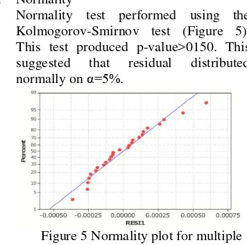
1. Normality

Normality test performed using the Kolmogorov-Smirnov test (Figure 5). This test produced p-value>0150. This suggested that residual distributed normally on α=5%.

Figure 5 Normality plot for multiple regression

Table 1 Distribution of frequency based on percentage interval of human trafficking victims in West Java.

Group

Interval of human trafficking victims

(%)

Districts/Municipalities

1 0.000000 – 0.000188 Bogor, Depok Municipality, Bekasi Municipality , Bekasi, Karawang, Subang, Indramayu, Cirebon Municipality, Kuningan, Ciamis, Banjar Municipality, Tasikmalaya Municipality , Tasikmalaya and Sukabumi Municipality. 2 0.000189 – 0.000352 Purwakarta, Cianjur, Bogor Municipality , Majalengka,

and Cirebon.

3 0.000353 – 0.000624 Sukabumi, Cimahi Municipality, Bandung Barat and Garut.

9

2. Homoskedasticity

Figure 6 is scatter diagram between residual and fitted value of multiple regression which have “horizontal

ribbon”. It exhibit that the assumption of homoskedasticity was fulfilled.

Figure 6 Scatter diagram between residual and the fitted value of multiple regression.

3. Independent error

The points in Figure 6 did not have a pattern so it could be concluded that the assumption of independent errors was fulfilled. Although the error in the regression were independent, testing for error with include spatial weighting matrix need to be done to knew whether they had spatial autocorrelation in these regression models. It could be done by

using Moran’s Index.

Testing for Spatial Effects

Testing for spatial effects were done to saw if there were spatial effects in data. Testing for spatial dependence used statistical Moran's Index. This test is a test of residual with included spatial weighting matrix. Moran's Index value = 0.48747 with p-value = 7.927e-05. This suggests that there was spatial autocorrelation in residual derived from the multiple regression model, so that need to be made a model that could accommodate spatial effects, namely spatial regression. In Figure 7 exhibit that there was spatial dependence effect on the dependent variable (Y) where there were a pattern of clustered data.

Figure 7 Moran’s scatterplot

Moran’s Index could also to identified spatial outliers, namely upper spatial outlier (hotspot) and under spatial outlier (coldspot). Base on Figure 7 there were upper spatial outliers (hotspots), they were exhibited as the numbered points 22, 18 and 1 in quadrant I at

Moran’s scatter plot. The numbered points were Cimahi Municipality, Bandung Municipality and Bandung District. Cimahi Municipality, Bandung Municipality and Bandung District had percentage of human trafficking victims above the average of others districts/municipalities. There were did not found the coldspots in quadrant III, it could be caused the percentage in quadrant III more uniform.

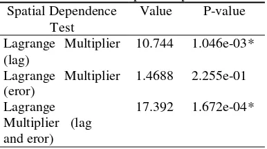
Once known proven that there were influenced of spatial effects, further step was to identified whether the type of spatial effects created. Spatial effects need to be identified were spatial dependence and spatial heterokedasticity. Testing for spatial dependence by using Lagrange Multiplier test (LM). This test was used to detect dependencies in lag, error, or both (lag and error). The results of spatial dependence could be seen in Table 2.

Table 2 The results of spatial dependence Spatial Dependence

Test

Value P-value

Lagrange Multiplier (lag)

10.744 1.046e-03* Lagrange Multiplier

(eror)

1.4688 2.255e-01 Lagrange

Multiplier (lag and eror)

17.392 1.672e-04*

*) Significant on α=0.05

According to Table 2 it could be seen that the p-value LM Lag = 1.046e-3 (less than α = 0.05). In conclusion reject H0. It means that

there was a lag of spatial dependence that need to be followed to creation of Spatial Autoregressive Model (SAR). Lagrange Multiplier lag and error could be used to identified the phenomena of combination, which identified dependence in lag and dependence in error between district/ municipality. Still based on Table 2 it could be seen that the p-value of LM lag and error=1.672e-4 (less than α = 0.05). The conclusion reject H0, it means that there were

a lag of spatial dependence in lag and error, so that need to be followed to creation of General Spatial Model too. Testing for spatial heterokedasticity by using Breush-Pagan Residual from regression

10

(BP). BP-value = 5.2897 where the p-value=6.247e-1 is greater than α = 0.05.

This test showed that there was no spatial heterokedasticity. It means that did not need using spatial regression models geog-raphically weighted.

Spatial Autoregressive Model (SAR)

Based on LM tests there was spatial lag dependence, this condition need to be continued to Spatial Autoregressive Model. Based on Table 3 it can be seen that the R2a =

57.45%, it means that the model able to explain the variation of the percentage of human trafficking victims until 57.45% and the remaining 42.55% is explained by other variables outside the model. Independent variables that significantly influences at α = 0.05 were X5 (the average of population with dead divorce status), X11 (the average of population with risen migrant status) and X13 (the average of population with maximum education in junior high school).

Table 3 The parameters estimation for SAR Variable Coefficient z P-value

ρ 6.288e-01 4.823 2.677e-4* Intercept 7.582e-04 0.262 7.927e-1 X2 -6.329e-06 -0.299 7.650e-1 X3 5.006e-04 0.321 7.480e-1 X4 -1.537e-02 -1.745 8.096e-2 X5 -1.640e-02 -3.460 5.400e-4* X8 -1.305e-05 -1.024 3.056e-1 X11 -7.475e-03 -3.856 1.152e-4* X13 8.186e-03 3.194 1.402e-3*

*) Significant α=0.05

R2a = 57.45% AIC-value = -356.7

SAR model is as follows:

̂

= 0.62879 WY + 0.0007582 - 0.0164030 X5-0.0074755 X11 + 0.00818620 X13. The value of autoregressive spatial lag

coefficient (ρ) obtained amounting 0.6288, it means that districts/municipalities had the highest percentage of human trafficking victims were suspected influenced by the districts/ municipalities that became their neighbors amounting 0.6288 multiplied by the average percentage of human trafficking victims in the districts/ municipalities around them with the assumption that the other variables fixed valuable. The assumptions test were also performed on SAR model. The assumptions that must be fulfilled were

normality, homoskedasticity and independent error. In this model all the assumptions were fulfilled (Appendix 4 and Appendix 5).

General Spatial Model (GSM)

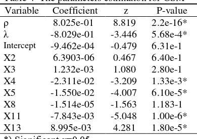
Based on LM tests there were spatial lag and error dependencies, so that need to be continued to General Spatial Model. According to Table 4 it could be seen that R2a

=71.34%, it means that the model was able to explain the variation of the percentage of human trafficking victims reach 71.34% and the remaining 28.66% is explained by the other variables outside the model. P-value

significant at α = 0.05 were variable X4 (the average of population with live divorce status), variable X5 (the average of population with dead divorce status), variable X11 (the average of population with risen migrant status) and variable X13 (the average of population with maximum education in junior high school).

Table 4 The parameters estimation for GSM Variable Coefficient z P-value

ρ 8.025e-01 8.819 2.2e-16*

λ -8.029e-01 -3.446 5.68e-4*

Intercept -9.462e-04 -0.479 6.31e-1

X2 6.3903-06 0.467 6.40e-1 X3 1.232e-03 1.080 2.80e-1 X4 -2.311e-02 -3.209 1.33e-3* X5 -1.550e-02 -4.007 6.10e-5* X8 -1.514e-05 -1.563 1.183-1 X11 -7.843e-03 -5.048 1.00e-6* X13 8.995e-03 4.281 1.80e-5*

*) Significant α=0.05

R2a= 71.34% AIC-value= -361.46

GSM model is as follows:

̂

= 0.80251WY - 0.80298 WU - 0.023112X4 -0.015506X5+0.0078429 X11 +

0.0089949 X13

11

human trafficking victims in the surrounding area. The spatial error coefficient (λ) amounting 0.8029 indicated that the error correlation between the district/municipality with other district/municipality that became their neighbors amounting 0.8029 multiplied by the average error in districts/municipalities that surround it. The assumptions test were also performed on GSM. The assumptions that must be fulfilled were normality, homoskedasticity and independent error. In this model all the assumptions were fulfilled (Appendix 6 and Appendix 7).

The Factors which Affected Percentage of Human Trafficking Victims in West Java

Before determining the factors that influenced the percentage of human trafficking victims in West Java, it was necessary to determined the best model with the indicator of goodness using of AIC-value (Akaike Information Criterion) which is a measure of the relative goodness of fit of a statistical model. It could be said to described the trade off between bias and variance in model construction, or loosely speaking between accuracy and complexity of the model. The smaller value of AIC could be said to get better model. In addition, the value of R2a could also be indicator of best model

selection. The comparison of AIC-value and R2a in multiple regression model, SAR and

GSM could be seen in Table 5.

Table 5 The indicators of goodness model

Indicator

Multiple Regression

Model

SAR

Model GSM AIC -345.41 -356.7 -361.46

R2a 38.42% 57.45% 71.34%

Based on Table 5 it could be concluded that the GSM is the best model for this case. In GSM model, the independent variables that affected the percentage of human trafficking victims were:

1. X4 = the average of population with live divorce status.

2. X5 = the average of population with dead divorce status.

3. X11 = the average of population with local migrant (risen migrant) status. 4. X13 = the average of population with

maximum education in junior high school.

Thus it could be seen that the factors affecting percentage of human trafficking victims in West Java in 2010 considering the influenced

of spatial districts/municipalities included divorce, local migrant (risen migrant) status and level of education.

CONCLUSIONS AND RECOMMENDATION

Conclusions

The percentage of human trafficking victims for certain district/municipality was influenced by the percentage of human trafficking victims in the surrounding districts/municipalities. Best model to modeling percentage of human trafficking victims in West Java in this study is General Spatial Model (GSM). The factors affecting percentage of human trafficking victims in West Java in 2010 by considering the influenced of spatial based on GSM as follows: the average of population with life divorce status, the average of population with dead divorce status, the average population with local migrant (risen migrant) status, and the average of population with maximum education in junior high school.

Recommendation

This study only used data in 2010 were handled by Integrated Service Center for Women and Children (ID). Further research should be done used previous and beyond year to see what factors are influential in each year. In addition, for the next research very recommended to use spatial poisson regression to compare the results.

REFERENCES

[AED] Academy for Educational Develop- ment. 2011. Indonesia. AED. [Internet].[downloaded 4 July 2012]. http://www.humantrafficking.org/countri es/indonesia.

Anselin L. 1988. Spatial Econometrics : Methods and Models, Kluwer Academic Publishers. Netherlands.

Anselin L. 1999. Spatial Econometrics. Dallas: University of Texas.

Arbia G. 2006. Spatial Econometrics: Statistical Foundation and Application

to Regional Convergence. Berlin:

Springer.

Belser P. 2005. Forced labour and human trafficking: Estimating the Profits. Chi G. 2008. The Impacts of Highway

12

An Integrated Spatial Approach.

Missisisppi: Missisisppi State University. Draper NR., Smith H.1992. Analisis Regresi

Terapan. Bambang Sumantri, translator. Jakarta: Gramedia Pustaka Utama-John Willey & Sons, Inc. .Translated from: Applied Regression Analysis.

Goździak EM., Bump MN, compiler. 2008.

Data and Research on Human Trafficking

[bibliography]. Washington DC: Georgetown University.

[IOM] International Organization for Migration (US). 2011. Case Data on Human Trafficking: Global Figures & Trends. United States: IOM.

Jabar tertinggi kasus trafficking. 2009. [Internet]. [downloaded 4 July 2012].

Seputar Indonesia. can be downloaded from:

http://www.gugustugastrafficking.org/ind ex.php?option=com_content&view=articl e&id=1140:jabar-tertinggi-kasus-trafficki ng&catid=134:info& Itemid=152. Laczko F. 2005. Data and Research on

Human Trafficking. International Migration 43(1/2):5-16.

LeSage JP. 1998. Spatial Econometrics [review]. Department of Economics University of Toledo.

LeSage JP., Pace RK.. 2011. Pitfalls in higher order model extensions of basic spatial regression methodology. Department of Finance and Economics Texas State University.

13

14

Appendix 1 The independent variables

The independent

Variable

The name of variable

X1

Population density in each district/municipality in West Java (people/km

2

)

X2 Sex ratio in each district/ municipality in West Java

X3 Average of population had married in each district/ municipality in West Java

X4 Average of population with live divorce status in each district/ municipality in West Java.

X5 Average of population with dead divorce status in each district/ municipality in West Java.

X6 Average of population who the first marriage <15years old in each district/municipality in West Java.

X7 Average of population who the first marriage more 25 years old in each district/ municipality in West Java

X8 Precentage of poor people in each district/municipality in West Java

X9 Average of people unemployment in each district/municipality in West Java. X10

Precentage of job seeker in each district/municipality in West Java

X11

Average of population with local migrant (risen migrant) status in each

district/municipality in West Java (persons)

X12

Average of population with maximum education in primary school in each

district/municipality in West Java (persons)

X13

Average of population with maximum education in junior high school in each

district/municipality in West Java (persons)

X14

Average of population with maximum education in high school in each

district/municipality in West Java (persons)

X15

Average of population had not been to school in each district/municipality in

West Java (persons)

X16

Average of population attending school in each district/municipality in West

Java (persons)

15

Appendix 2 Descriptive statistics of the independent variables

Variable Mean

Maximum Minimum

Value District/municipality Value District/municipality

X1 3512.846 14236.000 Bandung Municipality

559.000 Ciamis District

X2 102.945 107.150 Cianjur District 98.100 Ciamis District

X3 0.487 0.555 Ciamis District 0.432 Cirebon Municipality

X4 0.019 0.029 Subang District 0.010 Cirebon District

X5 0.043 0.066 Kuningan District 0.026 Depok Municipality

X6 0.047 0.094 Majalengka District 0.015 Bekasi Municipality

X7 0.030 0.068 Depok Municipality 0.008 Subang District

X8 11.371 20.710 Tasikmalaya Municipality

2.840 Depok Municipality

X9 0.045 0.076 Bogor Municipality 0.024 Banjar Municipality

X10 10.353 17.200 Bogor Municipality 5.120 Ciamis District

X11 0.043 0.115 Bekasi Municipality 0.008 Garut District

X12 0.322 0.484 Tasikmalaya District 0.144 Bekasi Municipality

X13 0.149 0.189 Cimahi Municipality 0.108 Cianjur District

X14 0.148 0.288 Bekasi Municipality 0.057 Tasikmalaya District

X15 0.063 0.173 Indramayu District 0.027 Bandung Municipality

X16 0.060 0.089 Bandung Municipality

0.042 Cianjur District

Information:

X1= The population density in each district/municipality in West Java (people/km2) X2 = Sex ratio in each district/ municipality in West Java

X3 = The average of population had married in each district/ municipality in West Java X4 = The average of population with live divorce status in each district/ municipality in

West Java.

X5 = The average of population with dead divorce status in each district/ municipality in West Java.

X6 = The average of population who the first marriage <15years old in each district/municipality in West Java.

X7 = The average of population who the first marriage more 25 years old in each district/ municipality in West Java

X8 = The precentage of poor people in each district/municipality in West Java X9 = The average of people unemployment in each district/municipality in West Java. X10 = The precentage of job seeker in each district/municipality in West Java

X11 = The average of population with risen migrant status in each district/municipality in West Java (persons)

X12 = The average of population with maximum education in primary school in each district/municipality in West Java (persons)

X13 = The average of population with maximum education in junior high school in each district/municipality in West Java (persons)

X14 = The average of population with maximum education in high school in each district/municipality in West Java (persons)

X15 = The average of population had not been to school in each district/municipality in West Java (persons)

16

Appendix 3 Fitting linear line pattern for the variables no-multicolinearity.

Scatterplot of Percentage of victims vs X4 Scatterplot of Percentage of victims vs X5 Scatterplot of Percentage of victims vs X3 Scatterplot of Percentage of victims vs X2

Scatterplot of Percentage of victims vs X8 Scatterplot of Percentage of victims vs X11

Scatterplot of Percentage of victims vs X13

17

Appendix 4 Normality plot for SAR model

Appendix 5 Scatter plot between residual and fitted value for SAR model

Appendix 6 Normality plot for GSM

Appendix 7 Scatter plot between residual and fitted value for GSM

Fitted value

18

Appendix 8 Administrative map of West Java Province