The Effect of Overdispersion on Regression Based Decision with Application to Churn Analysis on Indonesian Mobile Phone Industry

© EuroJournals Publishing, Inc. 2011 http://www.eurojournals.com/ejsr.htm

The Effect of Overdispersion on Regression Based Decision with

Application to Churn Analysis on Indonesian

Mobile Phone Industry

Asep Saefuddin

Department of Statistics, Faculty of Mathematics and Natural Sciences Bogor Agricultural University, Indonesia

E-mail: asaefuddin@gmail.com

Nur Andi Setiabudi

Innovation Center for Regional Resource Development and Community Empowerment (i-Crescent), Indonesia

E-mail: nurandi.mail@gmail.com

Noer Azam Achsani

Department of Economics and Graduate School of Management and Business Bogor Agricultural University, Indonesia

E-mail: achsani@yahoo.com; achsani@mb.ipb.ac.id

Abstract

Extra binomial variation or commonly known as overdispersion in logistic regression will provide incorrect conclusions. Overdispersion may be caused by the occurrence of variation in the response probabilities or correlation within the response variable. On the other hand, independent assumption of response variable is required in the logistic regression. In the case of correlated outcomes, although maximum likelihood gives unbiased estimates, their standard errors are underestimate.

This study was aimed at showing the effect of overdispersion on the hypothesis test of logistic regression. The example was taken from telecommunication industry to analyze churn of the subscribers. A simple method proposed by William was used to correct the effect of overdispersion by taking inflation factor into consideration. The result showed that the William method adjusted the standard error of estimates and provided more precise conclusion which was important in marketing strategies.

Keywords: Binomial logistic regression, overdispersion, William method, churn analysis

1. Introduction

non-Application to Churn Analysis on Indonesian Mobile Phone Industry 585

independent data is common phenomena, while the independence is a special case. Hence, clarifying the effect of overdispersion is necessary to obtain right conclusion.

If the response variable contains overdispersion, maximum likelihood produces unbiased estimates with narrow standard errors. As a result, effect of factors tends to be significant to the response variable. This situation is certainly unexpected and has to be avoided in decision making process in every industry. In the telecom industry, for example in churn modeling, the problem of overdispersion should get serious attention so that conclusions drawn provide correct insight on how the company’s strategy should be implemented.

The approach in handing overdispersion was introduced firstly by William (1982). William equates the value of Pearson’s chi-square statistic of the model to its approximate expected value in order to obtain the optimal weighting value for parameter estimation. In addition to William approch, there are many methods have been applied to handle overdispersion, for example, beta-binomial regression (Hajarisman and Saefuddin 2008; Kurnia et al 2002; Hinde and Demétrio 1998), mixed effect model (Handayani and Kurnia 2006) and logistics normal model (Hinde and Demétrio 1998). Overdispersion can also accommodated by using Quasi-likelihood method (Baggerly et al 2004) and double-exponential method approach (see Lambert and Roeder 1995).

In term of the application, many literatures have showed the overdispersion phenomenon in many areas, such as education (Hajarisman and Saefuddin 2008; Kurnia et al 2002), actuarial sciences (Cheong 2008; Ismail and Jemain 2005, 2007), bioinformatics (Lu et al 2005; Baggerly et al 2004) and biology (Etterson 2009; Rushton 2004; Lammertyn 2000; Hinde and Demétrio 1998).

In this paper we analyze the overdispersion phenomenon in Indonesian, especially in mobile phone industry -- a very dynamic market since Indonesia is a fast growing nation with more than 240 million inhabitants. Understanding the costumer behavior is in this sense a key element in order to win the competition. Logistic regression model is employed to analyze the loyalty of customer (commonly named as ‘subscriber’). Such approach is well-known as ‘churn analysis’ which is to predict ‘the churn of subscriber’. A subscriber is considered as churn when he (or she) stops his (or her) subscription from the company. Appropriate approach to handle the subscribers is very important as it is related to spending capital. Overdispersion in the mobile phone industries is common due to non independence of subscribers. The subscribers commonly tend to follow their group or community in using the services, i.e. because of the surrounding or collaborative effect (Ariely et al 2004) or social network effect.

This paper will be organized as follows. After the introduction in Section 1, we describe the data and methodology in Section 2. In this section, standard binary logistic model, overdispersion and how to handle overdispersion on binary logistic regression are reviewed. Section 3 provides the empirical results and discussion whereas Section 4 gives summary and concluding remarks.

2. Data and Methodology

2.1. Data

This study used call detail records (CDR) data taken from a well-known Indonesian mobile telecommunication provider to predict probability of a post-paid subscriber being churn at a certain time. This study involved 60 thousand phone numbers (MSISDNs) which were taken randomly from the database of the company. Each MSISDN consists of two explanatory variables namely ‘invoice’ and ‘tenure’. The invoice is monthly bill charged to subscriber related to the use of telecommunication service, while the tenure is a subscription period. Both of variables were stated in the categorical scale, in this case invoice consists of four categories and tenure consists of six categories. Thus, there would be (4  6) = 24 binomial observations (or k = 24).

churn. Meanwhile, if the MSISDN was still active, churn status would be zero (y=0). Among 60 thousand numbers, about 96.1% MSISDN still active until the next three months, while the 3.9% has churned.

In addition to estimating the standard logistic regression model, this study also examined the goodness of the model through deviance and Pearson’s chi-square statistic. If occurrence of overdispersion is found, William methods would be used to solve the problem. Furthermore, the results obtained by the William method were compared to the standard logistic regression.

2.2. Linear Logistic Regression

Suppose there are k binomial observations written in the form of ‘event (yi) / trial (ni)’ where yi is

number of occurrences of ‘success’ (event) and ni is number of replications (trial) on i-th observation (i

= 1, 2 , ..., k). Consider that i is probability of ‘success’ and E Y( )i i in is expected value for each

random variable, Yi. Logistic regression model which correspond every i with p explanatory variables, X1, X2, ..., Xp is:

0 1 1 2 2 0 1 1 2 2

exp( )

1 exp( )

i i p pi

i

i i p pi

X X X

X X X

                   

 ₍₁₎

In the linear form, the equation is often expressed as logit function of ‘success’, written as follow:

0 1 1

logit( ) log

1

i

i i p pi

i X X                

   ₍₂₎

where0, 1, 2, …, p are parameters of logistic regression model. The model is known as

Generalized Linear Model (GLM) with logit link function (McCullagh and Nelder 1989).

Parameters are estimated using maximum likelihood method, where its likelihood function is expressed as follows:

1

( ) i(1 )i i

k

i y n y

i i i i n L y      

 

 



 



(3) To obtain parameter estimates, ˆ, L() or logL() must be iterated to reach the maximum

value.

2.3. Deviance and Pearson’s Chi-Square

Deviance statistic measures lack of fit of the model. In a linear logistic regression model, if fitted value of number of ‘success’ denoted by

y

ˆ

i_{, where}

y

ˆ

i





ˆ

i

n

i_{, deviance statistics (D) is}





1

2 log log

ˆ ˆ

k

i i i

i i i

i i i i

y n y

D y n y

y n y

                     



(4) D statistic follows chi-square (2) distribution with k – p degree of freedom, where k is number

of binomial observations and p is numbers of parameters in the model. If fitted model is satisfactory, D statistic will be close to its number of degree of freedom. Or in other word, ratio of D statistic to its degree of freedom will be close to unity (Collett 2003).

Other approach to evaluate lack of fit of model is Pearson’s chi-square statistic, X2. It is obtained by the following formula:

2 2

1

ˆ

( )

ˆ (1 ˆ ) k

i i i

i _{i i i}

Application to Churn Analysis on Indonesian Mobile Phone Industry 587

2

X _{statistic follows chi-square (}2

) distribution with k – p degree of freedom. If fitted model is satisfactory, X2 statistic will be close to its number of degree of freedom, or ratio X2 statistic to its number of degree of freedom will be close to one (Collett 2003).

2.4. Over Dispersion

A logistic model is satisfactory if the ratio of D and X2statistic to number of degree of freedom is approximately one. When this ratio is significantly exceed one, assumption of binomial variation is invalid and overdispersion is occurred. Otherwise, a very rare phenomenon called underdispersion, presents when the ratio of D and X2 statistic to number of degree is smaller than one (Collett 2003). For more advanced method, Lambert and Roeder (1995) introduced a convexity or C plot and relative variance curve and relative variance test to examine overdispersion on Generalized Linear Model (GLM). Overdispersion diagnostics could be done also by a score test (Dean 1992).

Theoretically, overdispersion does not affect the parameter estimates of logistic models, but the standard errors of estimates are attenuated (Kurnia et al, 2002). Then, confidence interval of parameter will be narrow, causing the null hypothesis (H0 : i = 0) tend to be rejected. In other word, the

explanatory variables affect significantly to the response.

Modeling of overdispersion is often expressed in equation of variance of response variable, Yi,

as follow:





var( )Y_i 



_in_i(1



_i) 1 ( n_i 1)



(6) Where



1(ni 1)



_{is overdispersion’s scale and}  _{denote inflation factor. When}

overdispersion is not occurred or very small,  will equal to or approximately zero, so Yi exactly

follows binomial distribution, B(ni,pi), and var( )Yi ini(1i)(Collett 2003). However, when

overdispersion is existed,  exceeds zero and leads var(Yi) to be greater than i in (1i). Therefore the

actual variance of response variable is greater than the variance calculated from binomial distribution.

2.5. William Method

Parameter estimate of , denoted by ˆ, is obtained by equating X2statistic of the model to its approximate expected value, written as :

2 2

1

ˆ

( )

ˆ (1 ˆ )

k

i i i i i _{i i i}

w y n

X n       



and

 

2





1

(1 ) 1 ( 1)

k

i i i i i

i

E X w w v d  n



  





(7) where vi i in(1i)_{, wi is the weight and vi is diagonal element of the variance-covariance matrix}

of the linear predictor, ˆi ˆjxji_{. The value of} X2 _{statistic depends on} ˆ_{, so iteration process is}

needed to find optimum value. This procedure was firstly introduced by William (1982), and then called William method. The algorithm of William method is described as follow.

1. Assumed



0, calculate parameter estimate of logistic regression model, ˆ, using maximum likelihood method. Calculate the X2 statistics of fitted model.

2. Compared X2 statistics to 2 (k p)



 _{distribution. If} 2

X _{statistic is too large, conclude that}

0

 _{and calculated initial estimates of  using following formula :}





0

2

1

ˆ ( )

( 1)(1 )

k

i i i

i

X k p

n v d





  

 

3. Using initial weight 0 0

ˆ 1 ( 1)

i i

w  _ n 



_

, recalculate the value of ˆ dan X2statistic.

4. If X2_{statistic closes to its number of degree of freedom,} k p_{, estimated value of}  _is

sufficient. If not, re-estimate  using following expression:









2

1

1

1

ˆ (1 )

( 1)(1 )

k

i i i i i

k

i i i i i i

X w w v d

w n w v d

  



 

 





₍₉₎

If X2_{statistic remain large, return to step 3 until optimum value of estimated}  _obtained.

Once  has been estimated by ˆ, wi 1 1 (



 ni1)



_{could be used as weights in fitting new} model (Collett 2003; William 1982).

3. Results and Discussion

3.1. Result of Standard Logistic Regression

Setiabudi and Saefuddin (2009), conducted a logistic regression model to estimate the probability of each subscriber being churn based on invoice and tenure following linear form of

0 1* 2*

logit (_jk)  invoice tenure

Invoice and tenure were recorded in categorical scales; hence these two variables were transformed into dummy variables. The parameterization was done using reference method (see SAS Institute, 2009). In this case, the last category of each explanatory variable was reference for other categories. Thus, the 4th category of invoice i.e. subscribers who spent more than IDR150,000 a months in using telecommunication services, written as invoice4, would be reference for invoice1, invoice2, and

invoice3; while tenure6 i.e. subscribers who have been subscribed for 60 months or more, would be a

reference for the tenure1 until tenure5. Table 1 shows completely how explanatory variables were

categorized.

Using standard logistic regression, parameter estimates of model were listed in Table 2, and evaluations to goodness of this model were in Table 3.

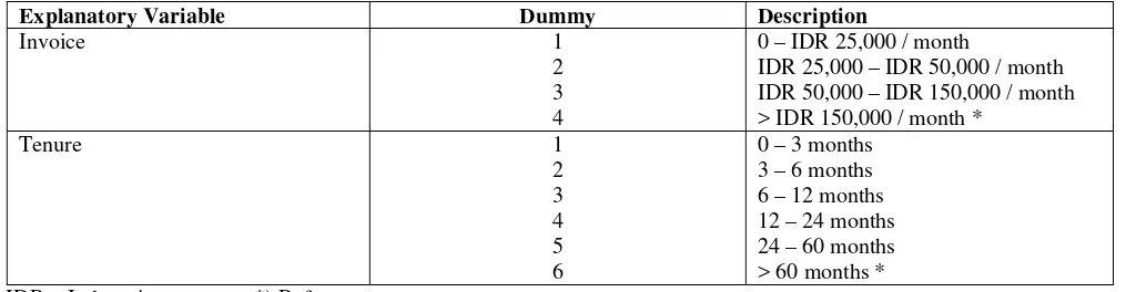
Table 1: Explanatory variables and their dummy variables

Explanatory Variable Dummy Description

Invoice 1 0 – IDR 25,000 / month

2 IDR 25,000 – IDR 50,000 / month 3 IDR 50,000 – IDR 150,000 / month 4 > IDR 150,000 / month *

Tenure 1 0 – 3 months

2 3 – 6 months 3 6 – 12 months 4 12 – 24 months 5 24 – 60 months 6 > 60 months * IDR = Indonesian currency *) Reference

Table 2: Parameter estimates of model using standard logistic regression

Explanatory Variable



ˆ SE( )ˆ df p-value

Intercept –5.708 0.107 1 <.0001

Invoice 3

Invoice1 0.816 0.097 1 <.0001

Application to Churn Analysis on Indonesian Mobile Phone Industry 589

Table 2: Parameter estimates of model using standard logistic regression - continued

Invoice3 0.399 0.063 1 <.0001

Tenure 5

Tenure1 3.710 0.109 1 <.0001

Tenure2 3.038 0.113 1 <.0001

Tenure3 2.147 0.121 1 <.0001

Tenure4 2.481 0.113 1 <.0001

Tenure5 0.724 0.119 1 <.0001

The value of deviance statistic was 182.849 with 15 degree of freedom and the value of Pearson’s chi-square was 186.919 with 15 degree of freedom, indicated the churn data contained overdispersion. This phenomenon was reasonable since the behavior of a person to subscribe to a mobile phone service provider depend on, or affected by, other persons or community in the same groups or segments. Therefore the response variable was not independent or there was correlation between subscribers within binomial observation.

Table 3: Goodness of fit of standard logistic regression model based on deviance and Pearson’s chi-square statistic

Statistic Value df Value/df p-value

Deviance 182.849 15 12.190 <.0001 Pearson’s chi square 186.919 15 12.461 <.0001

3.2. Result of Weighted Logistic Regression Model Using William Method

Since overdispersion occurred, William method will be used to estimate weighted logistic regression. Through iteration process, estimated parameter of inflation factor, ˆ, was found to be 0.008657, thus overdispersion scale or weights was wi 1 1 0.008657(  ni1)_{, where ni denotes number of} subscribers in the i-th group. Using weights of wi we obtained new logistic model, namely weighted

logistic regression model using William method, whose parameter estimates presented on Table 4. Furthermore, the goodness of this model according to deviance and Person’s chi-square statistic was given by Table 5.

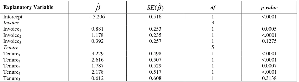
Table 4: Parameter estimates of weighted logistic regression model using William method

Explanatory Variable



ˆ SE( )ˆ df p-value

Intercept –5.296 0.516 1 <.0001

Invoice 3

Invoice1 0.881 0.253 1 0.0005

Invoice2 1.178 0.235 1 <.0001

Invoice3 0.392 0.257 1 0.1275

Tenure 5

Tenure1 3.229 0.498 1 <.0001

Tenure2 2.616 0.507 1 <.0001

Tenure3 1.787 0.529 1 0.0007

Tenure4 2.178 0.517 1 <.0001

Tenure5 0.612 0.608 1 0.3138

Table 5: Goodness of weighted logistic regression model with William method based on deviance and Pearson’s chi-square statistic

Statistic Value df Value/df p-value

Deviance 15.443 15 1.030 0.4200

The William method corrected the goodness of fit of model indicated by the value of deviance and Pearson’s chi square statistic. The value of deviance (D=15.443) and Pearson’s chi-square (X2=15.443) which very close to their degree of freedom (df=15).

In the weighted logistic regression model with William method, invoice3 and tenure5 did not

significantly differ from zero (Table 4). Whereas, parameter estimates of the standard logistic regression model were all significant at 95% confidence interval (Table 1). Since a standard logistic regression model did not accommodate overdispersion, the value of SE would be underestimated, thus decision making about relationship of explanatory variables and corresponding response variable would be invalid. In other hand, William method provided a larger SE of estimates, as a result of adjustment to extra binomial variation within data (Kurnia et al, 2002).

3.3. Best Model Selection

When parameter estimate of invoice3 did not significantly differ, the model can be simplified by

joining invoice3 and its reference, invoice4, thus all subscribers who had invoice more than IDR50,000

were classified as one category. The same way applied for tenure5 and tenure6. Thus, the invoice would

consist of three categories while the tenure consists of five categories where the last category of each variable was reference of other categories.

Using the modified categories, standard logistic regression was implemented to estimate a new model with D=164.571 on df=8 and X2=163.129 on 8. Thus, overdispersion was still existed and the model might be not appropriate. Hence, the William method applied, and then obtained

ˆ _0.009347

  _{which equivalent with the weights of}wi 1 1 0.009347*(  ni1)_{. Since D=8.649 on} df=8 and X2=8.000 on 8, the model whose parameter estimates presented on Table 6 was satisfactory.

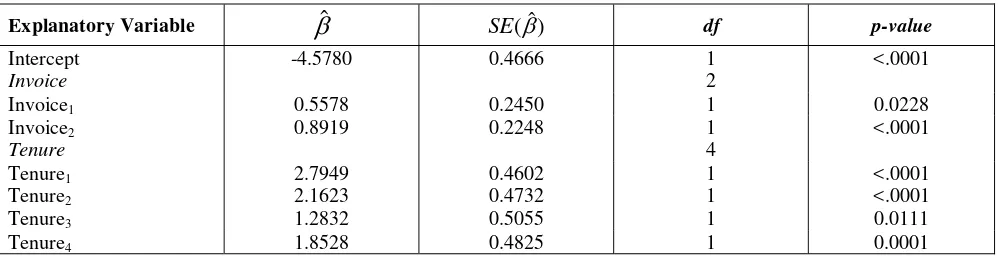
Table 6: The modified model of weighted logistic regression using William method

Explanatory Variable



ˆ SE( )ˆ df p-value

Intercept -4.5780 0.4666 1 <.0001

Invoice 2

Invoice1 0.5578 0.2450 1 0.0228

Invoice2 0.8919 0.2248 1 <.0001

Tenure 4

Tenure1 2.7949 0.4602 1 <.0001

Tenure2 2.1623 0.4732 1 <.0001

Tenure3 1.2832 0.5055 1 0.0111

Tenure4 1.8528 0.4825 1 0.0001

The model on Table 4 called original model, while the modified model is on Table 6. The later model produced satisfactory result and looked simpler than the original one. Practically the modified model might recommend more efficient guidance on how the marketing strategies have to be performed to minimize the occurrence of subscribers churn. In addition, the AIC (Akaike Information Criterion) statistic was employed to obtain the best between the original and modified model following Agresti (2007) and McCullagh and Nelder (1989). Based on the AIC statistics, the modified model was better than the original one, i.e. the AIC statistics of modified model was 855.54 while the AIC statistics of the original one was 1183.97.

4. Concluding Remarks

Application to Churn Analysis on Indonesian Mobile Phone Industry 591

In the case of churn analysis in the Indonesian telecommunication industry, model with overdispersion will recommend a misleading marketing strategy. It was shown that if overdispersion ignored, statistical recommendations slightly distorted. In the example, standard logistic regression found that all the category of invoice and tenure looks significant. After correction to overdispersion, there were several categories of invoice which were actually in one category. Likewise, there were several categories of tenure which were actually in one category. Relation to marketing strategy, other than this distortion will cause wastage due to excessive cost allocation and inappropriate strategy. Correcting the overdispersion will provide simple and appropriate marketing campaign efficiently and effectively.

References

[1] Agresti, A. (2007) An Introduction to Categorical Data Analysis, Second edition. John Wiley & Sons, New Jersey, US.

[2] Ariely, D., J.G. Lynch and M. Aparicio (2004) Learning by collaborative and individual-based recommendation agents. Journal of Consumer Psychology 14(1): 81–94.

[3] Baggerly, K.A., L. Deng, J.S. Morris and C.M. Aldaz (2004) Overdispersed logistic regression for SAGE: modelling multiple groups and covariates. BMC Bioinformatics 5:144. http://www.biomedcentral.com/1471-2105/5/144

[4] Cheong, P.W., A.A. Jemain and N. Ismail (2008) Practice and pricing in non-life insurance: the malaysian experience. Journal of Quality Measurement and Analysis 4(1): 11-24.

[5] Collett, D. (2003) Modelling Binary Data, Second edition. Chapman & Hall/CRC, London, UK.

[6] Dean, C.B. (1992) Testing for overdispersion in poisson and binomial regression models. Journal of the American Statistical Association 87(418) : 451-457.

[7] Etterson, M.A., G.J. Niemi and N.P. Danz (2009) Estimating the effects of detection heterogeneity and overdispersion on trends estimated from avian point counts. Ecological Applications 19(8): 2049–2066.

[8] Hajarisman, N. and A. Saefuddin (2008) The beta-binomial multivariate model for correlated categorical data. Jurnal Statistika 8(1): 61–68.

[9] Handayani, D. and A. Kurnia (2006) Mixed effect model approach for logistic regression model with overdispersion. Proceeding of ICoMS-1, Bandung 19-21 June 2006.

[10] Hinde, J. and C.G.B. Demétrio (1998) Overdispersion: models and estimation. Computational Statistics and Data Analysis 27: 151-170.

[11] Ismail, N. and A.A. Jemain (2005) Generalized poisson regression: an alternative for risk classification. Jurnal Teknologi 43(C): 39–54.

[12] Ismail, N. and A.A. Jemain (2007) Handling overdispersion with negative binomial and generalized poisson regression models. Proceeding of Casualty Actuarial Society Forum, Winter 2007 Edition : 103 – 158.

[13] Kurnia, A., A. Saefuddin and E. Sutisna (2002) Overdispersi dalam regresi logistik. Proceeding of Seminar Nasional Statistika, Bogor, 28 September 2002 : 11-17.

[14] Lambert, D. and K. Roeder (1995) Overdispersion diagnostics for generalized linear models. Journal of the American Statistical Association 90(432): 1225-1236.

[15] Lammertyn, J., M. Aerts, B.E. Verlinden, W. Schotsmans and B.M. Nicolaï (2000) Logistic regression analysis of factors influencing core breakdown in ‘Conference’ pears. Postharvest Biology and Technology 20: 25–37.

[17] McCullagh, P., and J.A. Nelder (1989) Generalized Linear Models, Second ed. Chapman and Hall, London, UK.

[18] Rushton, S.P., S.J. Ormerod and G. Kerby (2004) New paradigms for modelling species distributions? Journal of Applied Ecology 41: 193–200.

[19] SAS Institute Inc. (2009) SAS/STAT® 9.2 User’s Guide, Second Edition, SAS Institute Inc., Cary, NC, US.

[20] Setiabudi, N.A. and A. Saefuddin (2009) Customer segmentation and churn analysis in the mobile telecommunications industry, Book of Abstract ICCS-X Conference, Cairo, December 20–23, 108.