Performance Analysis of Covariance Matrix
Estimates in Impulsive Noise
Frédéric Pascal, Philippe Forster
, Member, IEEE
, Jean-Philippe Ovarlez, and Pascal Larzabal
, Member, IEEE
Abstract—This paper deals with covariance matrix estimates in impulsive noise environments. Physical models based on com-pound noise modeling [spherically invariant random vectors (SIRV), compound Gaussian processes] allow to correctly describe reality (e.g., range power variations or clutter transitions areas in radar problems). However, these models depend on several unknown parameters (covariance matrix, statistical distribution of the texture, disturbance parameters) that have to be estimated. Based on these noise models, this paper presents a complete anal-ysis of the main covariance matrix estimates used in the literature. Four estimates are studied: the well-known sample covariance matrix MSCM and a normalized version M , the fixed-point (FP) estimateMFP, and a theoretical benchmarkMTFP. Among these estimates, the only one of practical interest in impulsive noise is the FP. The three others, which could be used in a Gaussian context, are, in this paper, only of academic interest, i.e., for comparison with the FP. A statistical study of these estimates is performed through bias analysis, consistency, and asymptotic distribution. This study allows to compare the performance of the estimates and to establish simple relationships between them. Finally, theoretical results are emphasized by several simulations corresponding to real situations.
Index Terms—Asymptotic distribution, bias, consistency, covari-ance matrix estimates, non-Gaussian noise, spherically invariant random vectors (SIRV), statistical performance analysis.
I. INTRODUCTION
I
T IS often assumed that signals, interferences, or noises are Gaussian stochastic processes. Indeed, this assump-tion makes sense in many applicaassump-tions. Among them, we can cite sources localization in passive sonar where signals and noises are generally assumed to be Gaussian, radar detection where thermal noise and clutter are often modeled as Gaussian processes, and digital communications where the Gaussian hypothesis is widely used for interferences and noises.In these contexts, Gaussian models have been thoroughly in-vestigated in the framework of statistical estimation and de-tection theory [1]–[3]. They have led to attractive algorithms.
Manuscript received January 24, 2007; revised September 18, 2007. The as-sociate editor coordinating the review of this manuscript and approving it for publication was Prof. Steven M. Kay.
F. Pascal is with SATIE, ENS Cachan, UMR CNRS 8029, 94235 Cachan Cedex, France (e-mail: [email protected]).
P. Forster is with the Groupe d’Electromagnétisme Appliqué (GEA), Institut Universitaire de Technologie de Ville d’Avray, 92410 Ville d’Avray, France (e-mail: [email protected]).
J.-P. Ovarlez is with the French Aerospace Lab, ONERA, DEMR/TSI, BP 72, 92322 Chatillon Cedex, France (e-mail: [email protected]).
P. Larzabal is with the IUT de Cachan, C.R.I.I.P, Université Paris Sud, 94234 Cachan Cedex, France, and also with the SATIE, ENS Cachan, UMR CNRS 8029, 94235 Cachan Cedex, France (e-mail: [email protected]).
Color versions of one or more of the figures in this paper are available online at http://ieeexplore.ieee.org.
Digital Object Identifier 10.1109/TSP.2007.914311
For instance, we can cite the stochastic maximum-likelihood method for sources localization in array processing [4], [5], and the matched filter in radar detection [6], [7] and in digital com-munications [8].
However, such widespread techniques are suboptimal when the noise process is a non-Gaussian stochastic process [9]. There-fore, non-Gaussian noise modeling has gained many interest in the last decades and currently leads to active researches in the literature. High-order moment methods [10] have initiated this research activity and particle filtering methods [11] are now in-tensively investigated. In radar applications, experimental clutter measurements, performed by Massachusetts Institute of Tech-nology (MIT, Cambridge) [12], showed that these data are not correctly described by Gaussian statistical models. More gen-erally, numerous non-Gaussian models have been developed in several engineering fields. For example, we can cite the -dis-tribution already used in the area of radar detection [13], [14]. Moreover, let us note that the Weibull distribution is a widely spread model in biostatistics and in radar detection [15].
One of the most general and elegant impulsive noise model is provided by the so-called spherically invariant random vectors (SIRVs). Indeed, these processes encompass a large number of non-Gaussian distributions, included, of course, Gaussian pro-cesses and also, the aforementioned distributions. SIRVs and their variants have been used in various problems such as ban-dlimited speech signals [16], radar clutter echoes [17], [18], and wireless radio fading propagation problems [19], [20]. More-over, SIRVs are also connected to other interesting processes such as the “heavy-tailed” processes, which have been used to model impulse radio noises as well as processes used in finan-cial engineering models [21].
A SIRV is a compound process. It is the product of a Gaussian random process with the square root of a nonnegative random scalar variable (called thetexturein the radar context). Thus, the SIRV is fully characterized by the texture (representing an un-known power) and the unun-known covariance matrix of the zero-mean Gaussian vector. One of the major challenging difficulties in SIRV modeling is to estimate these two unknown quantities [22]–[24]. These problems have been investigated in [25] for the texture estimation while [26] and [27] have proposed different es-timates for the covariance matrix. The knowledge of the eses-timates statistical properties is essential to use them in different contexts. This paper deals with three covariance matrix estimates: the well-known sample covariance matrix (SCM) [28], the theoret-ical fixed point (TFP), both studied for academic purposes, and the fixed point (FP), which may easily be implemented in prac-tice [29]. These three estimates arise as solutions of maximum-likelihood (ML) or approximate maximum-maximum-likelihood (AML) problems. The main contribution of this paper is to derive and
to compare their statistical properties: bias, consistency, second-order moment, and asymptotical distribution.
This paper is organized as follows. In Section II, a background on the SIRV covariance matrix estimates is given. Sections III–V present the main results of this paper, i.e., performance analysis of the estimates in terms of bias, consistency, covariance matrices, and asymptotic distribution. For clarity, long proofs are reported in Appendices A–E. Finally, Section VI gives some simulation results confirming the theoretical analysis.
II. PROBLEMFORMULATION
In this section, we introduce the SIRV noise model under study and the associated covariance matrix estimates. In the fol-lowing, denotes the conjugate transpose operator, denotes the transpose operator, stands for the statistical mean of a random variable, and is the trace of the matrix .
A. Statistical Framework
Let us recap some SIRV theory results. An SIRV is a com-plex compound Gaussian process with random power. More precisely, an SIRV [30], [31] is the product between the square root of a positive random variable and an -dimensional in-dependent zero-mean complex Gaussian vector
For identifiability considerations, the covariance matrix is normalized according to (see [26]) and called, in the sequel, normalization #1.
The SIRV probability density function (pdf) expression is
where is the texture pdf.
Notice that, when is Dirac distributed, i.e.,
, the resulting SIRV is a zero-mean Gaussian vector with co-variance matrix , while when is Gamma distributed, the resulting SIRV is the well-known -distribution. However, the closed-form expression of the texture pdf is not always avail-able (e.g., Weibull SIRV). Thus, in problems where is un-known and has to be estimated from SIRV realizations, it would be of interest to have a covariance matrix structure estimate in-dependent of the texture.
B. Covariance Matrix Structure Estimation
The covariance matrix has to be normalized to identify the SIRV noise model. Consequently, it is reasonable to think that the same normalization has to be applied to its estimate. How-ever, as it will be shown later, the appropriate normalization for
performance analysis is and will be called
normalization #2 for any estimate of
Normalization #1:
Normalization #2: or, equivalently,
.
(1) When is unknown, it could be objected that normaliza-tion #2 is only of theoretical interest while only normalizanormaliza-tion
#1 can be applied in practice. In most applications, however, is exploited in such a way that any scale factor on has no influence on the final result. (e.g., in radar detection, the de-tector could be a likelihood ratio, homogeneous in terms of [26]). This would also be the case in general estimation prob-lems where estimated parameters only depend on the structure of the covariance matrix. Hence, the normalization, chosen for any studied case, is of little importance.
In this framework, the three estimates will be built from independent realizations of denoted
and called secondary data.
First, if we had access to the independent realizations of the underlying Gaussian vector , the ML estimate would lead to the SCM, which is Wishart distributed [33] and defined by
(2)
However, in practice, we only have access to the inde-pendent realizations of an SIRV and it is impos-sible to isolate the Gaussian process . However, it is used as a benchmark for comparison with the other estimates. More-over, performance analysis will lead to an interpretation of the theoretical expressions obtained for the other estimates.
To fulfill normalization #2, will be defined by
(3)
Equation (3) can also be written
(4)
Estimates (2) and (3) have only a theoretical interest since the ’s are not available. Practical estimates are functions of the ’s and “good” ones should not depend on the ’s.
A first candidate is the normalized sample covariance matrix (NSCM) [34] given by
which can be rewritten only in terms of ’s
As the statistical performance of this estimate has been exten-sively studied in [35], only its statistical analysis results will be presented in order to compare all available estimates. Moreover, although this “heuristic” estimate respects normalization #1, it exhibits several severe drawbacks.
A second candidate, provided by the ML theory [26], [27], is the FP estimate of , defined as an FP of function
where positive definite with matrices with elements in .
The notation stresses the dependency on and on the covariance matrix involved in the ’s.
As shown in [36], equation has a solution
of the form , where is an arbitrary scaling factor. In this paper, the only solution satisfying normalization #2 is called the FP estimate. In other words, is the unique solu-tion of
(6)
such that respects normalization #2.
Notice that , as , does not depend on the texture as emphasized in (6).
Remark II.1: The FP is the ML estimate when the texture is assumed to be an unknown deterministic parameter and is an AML when is assumed to be a positive random variable [26], [27].
Finally, an analysis of another texture-independent estimate of is performed, where
(7)
In this paper, it is called the TFP estimate. This estimate is only of theoretical interest since it depends on the unknown co-variance matrix . It is closely related to the FP estimate (6) and it will be shown that its statistical performance has strong connections with those of . Notice that satisfies
normalization #2: ; so the TFP estimate
will be considered as the benchmark for .
In this context of covariance matrix estimation in impulsive noise, the statistical properties of the three proposed estimates , , and will be established in this paper, while existing results concerning and will be reminded.
III. BIASANALYSIS
This section provides an analysis of the bias denoted by
for each estimate introduced previously.
The SCM has been studied in literature and is unbi-ased. Now, bias will be analyzed next. Its unbiasedness is presented in the following theorem.
Theorem III.1 (Unbiasedness of ): is an unbiased estimate of .
Proof: To prove that , the focus is put on
(8)
For this purpose, let us whiten the ’s in (8), according to
(9)
For , are given by
(10)
Since for any , the th element of
de-noted by can be written as
where for and ,
and , where denotes the Chi-squared
distribution with two degrees of freedom and , the uniform distribution on interval , and and are independent.
Thus, by replacing the ’s in (10), element of matrix is
Since , for any , the nondiagonal
el-ements of are null. Then, diagonal element is
is a Beta of the first kind distributed random variable with parameters 2 and .
Moreover, the statistical mean of a is
, thus for
and for and . Using these
results in (9) leads to
The analysis of bias is provided in two cases. In the most general case, Theorem III.2 gives a closed-form expression of bias. Then, Theorem III.3 proves the unbiasedness
of when , where is the identity matrix.
Theorem III.2 ( Bias When Has Distinct Eigen-values): Assuming that has distinct eigenvalues,
bias is given by
where the following are true:
• the operator reshapes a -vector into
a diagonal matrix with elements
;
• is the orthogonal matrix of the eigenvectors of ;
• with
if and if , where is
the eigenvalue of ;
• with .
Proof: See [35].
Theorem III.3 (Unbiasedness of When ):
is an unbiased estimate of
Proof: With the same reasoning as in Theorem III.1’s proof, it is shown that is a diagonal matrix with elements
where is a Beta of the first kind
distributed random variable with parameters 2 and . Since
the statistical mean of a is ,
, which completes the proof.
Theorem III.4 (Unbiasedness of ): is an unbiased estimate of
Proof: For clarity, in this section, will be denoted . The first part of the proof is the whitening of the data. By applying the following change of variable, to (6), one has
where
Therefore
is thus the unique FP estimate (up to a scaling factor) of the identity matrix. Its statistics are clearly independent of
since the ’s are .
Moreover, for any unitary matrix
where are also independent identically distributed (i.i.d.) . Therefore, has the same distribution as
, so
for any unitary matrix
Since is different from , Lemma A.1, detailed in Appendix A, ensures that . Moreover, since
, thus ; also, since
, .
In conclusion, is an unbiased estimate of , for any in-teger .
Theorem III.5 (Unbiasedness of ): is an unbi-ased estimate of
Proof: To prove Theorem III.5, changing variable
, where , leads to
The equality
is proven by Theorem III.3.
Thus, , i.e., is an unbiased estimate
of .
IV. CONSISTENCY
An estimate of is consistent if
where is the number of secondary data ’s used to estimate and stands for any matrix norm.
Remark IV.1: When has distinct eigenvalues, Theorem III.2 shows that is a biased estimate of . Moreover, this bias does not depend on the number of ’s. Thus, is not a consistent estimate of . In the sequel, since suffers from the previous drawbacks (biased and nonconsistent), thus from here on, this estimate will not be taken into account when has distinct eigenvalues. On the other hand, the NSCM estimate of will be studied as a particular case of the TFP estimate.
Under Gaussian assumptions, the SCM estimate is consistent. This result was established in [28, pp. 80–81].
Theorem IV.1 ( consistency): is a consistent esti-mate of .
Proof: By whitening the ’s in (4)
Then, the weak law of large numbers (WLLN) demonstrates that
Finally, basic theorems on stochastic convergence show that
which means that is a consistent estimate of .
Theorem IV.2 ( Consistency): is a consistent es-timate of .
Proof: See Appendix B.
Theorem IV.3 ( Consistency): is a consistent estimate of .
Proof: Theorem III.1 and the WLLN imply that is a consistent estimate of .
V. ASYMPTOTICDISTRIBUTION
A. Notations
In this section, a perturbation analysis will be used to derive the asymptotic distribution of the three estimates, all denoted for clarity. For this purpose, is rewritten as
The essential quantities for the analysis are defined as fol-lows:
• ;
• , where is the vector containing all the ele-ments of and denotes the operator which reshapes the matrix elements into an column vector. In the sequel, these quantities will be indexed according to
the studied estimate: , , , and .
The asymptotic distribution of is obtained from the distri-bution of with the following Proposition.
Proposition V.1:
where represents the Kronecker product.
Proof: . This is proven by the
property for any matrix , ,
and (see [33, p.9]).
The aim of this section is to derive the asymptotic distribution of , i.e., the asymptotic distribution of , where denotes the real part of the complex vector and is its imaginary part. It will be shown later that this distribution is Gaussian and therefore is fully characterized by its asymptotic covariance matrix. This matrix may be derived from the two quantities and . However, in this specific case, is the of a Hermitian matrix so can be obtained
from .
B. Results
The following original results use the notations and , defined by
(11)
(12)
where is defined by, for ,
for
for and
else.
(13) The covariance matrix of has been established in [28] and is reminded here.
Theorem V.1 ( Asymptotic Distribution):
1) , where stands
for the convergence in distribution and denotes the covariance matrix of , which can be straightfor-wardly obtained from the following.
2) , where is defined above.
3) .
Proof: See [33].
Theorem V.2 ( Asymptotic Distribution):
1) , where denotes the
covariance matrix and can be straightforwardly obtained from the following.
2) .
3) .
The two matrices and are defined by (11) and (12).
Proof: See Appendix C.
Theorem V.3 ( Asymptotic Distribution):
1) , where
de-notes the covariance matrix and can be straightforwardly obtained from: the following.
2) .
3) .
Proof: See Appendix D.
In [37], the following original results on with the pre-vious notations have been partially established.
Theorem V.4 ( Asymptotic Distribution):
1) , where denotes the
covariance matrix and can be straightforwardly obtained from the following.
2) .
3) .
Proof: Proof of Theorem V.4 is fully given in Appendix E.
C. Synthesis
All the results on the asymptotic second-order moment of are recapped in Table I.
• The three estimates , , and share the same asymptotic covariance matrix up to scaling factors.
• More precisely, ,
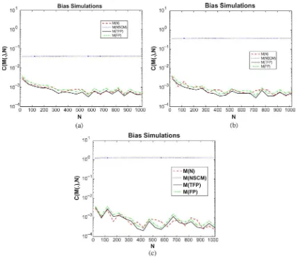
Fig. 1. Estimates bias for different values of: (a) = 0:1; (b) = 0:5; and (c) = 0:9.
TABLE I
ASYMPTOTICSECOND-ORDERMOMENT
same asymptotic distribution. Therefore, , with secondary data, has the same asymptotic behavior as
, with secondary data. Since
is the SCM up to a scale factor, we may conclude that, in problems invariant with respect to a scale factor on the covariance matrix, the FP estimate is asymptotically equivalent to the SCM with a little less secondary data:
data.
VI. SIMULATIONS
In order to enlighten results provided in Sections III–V, some simulation results are presented. Since and are
texture independent and and are only valid under Gaussian assumption, simulations are performed with Gaussian noise.
Operator is defined as the empirical mean of the quantities obtained from Monte Carlo runs. For each iteration , a new set of secondary data is generated to
com-pute .
Thus, for example, is defined by
A. Bias Analysis
The results presented in this section are obtained for complex Gaussian zero-mean data with covariance matrix defined by
for
Fig. 1 shows the bias of each estimate for different values of
: , and . The length of each vector is .
For that purpose, a plot of versus the
number of ’s and for any matrix norm, is presented for each estimate.
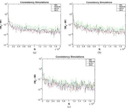
Fig. 2. Estimates consistency for different values of.m = 3. (a) = 0:1; (b) = 0:5; and (c) = 0:9.
value of , while the bias of (when the covariance matrix is different from ) does not tend to zero with the number of ’s. Moreover, this simulation underlines the fact that bias does not depend on ; it is constant for all
number of ’s.
Furthermore, the correlation coefficient has, of course, no influence on the unbiased estimates. On the other hand, for each value of , the bias of the NSCM estimate is different and it tends to 0 when tends to 0 (case tends to ).
B. Consistency Analysis
Fig. 2 presents results of estimates consistency. For that
pur-pose, a plot of versus the number of
’s is presented for each estimate.
It can be noticed that the previous criterion tends to 0 when tends to , for each estimate and each value of . However, there are more fluctuations when data are strongly correlated (i.e., ).
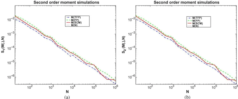
C. Second-Order Moment Analysis
Simulations relating to second-order moment have been rep-resented on two different graphics: one on transpose operator
results and the other for the transpose conjugate operator results.
In Fig. 3, the quantity
is plotted for the four studied estimates versus the number of ’s, where is defined in the notations used in Section V and the matrix represents the closed-form expression of
for the different estimates.
Let us recall the following results:
• for , ;
• for , ;
• for , ,
• for , ;
where is defined by (11) and by (13).
Fig. 3(a) validates results on second-order moment estimates obtained in Section V because the quantity tends to zero when tends to infinity for all estimates.
From Fig. 3(b), the same conclusion as Fig. 3(a) is drawn but with the transpose conjugate operator , i.e.,
Fig. 3. Estimates second-order moment: (a) transpose case and (b) transpose conjugate case.
VII. CONCLUSION
In this paper, the problem of covariance matrix estimation in impulsive noise modeled by SIRVs was considered. Four
estimates , , , and have been studied
through a theoretical statistical analysis: bias, consistency, asymptotic distribution, and second-order moments. All orig-inal results have been illustrated by simulations.
In this impulsive noise context, the SCM cannot be used in practice since this estimate of the Gaussian kernel is based on unavailable data. The same remark holds for the TFP estimate as it depends on the unknown covariance matrix that needs to be estimated. Finally, the well-known NSCM is biased and not con-sistent. Therefore, the only appropriate estimate is the so-called FP estimate, which is unbiased, consistent, and has, up to a scale factor, the same second-order moments as the SCM of the Gaussian kernel.
Finally, this statistical study will allow a performance anal-ysis of signal processing algorithms based on these estimates. For instance, performance of radar detection algorithms using the FP estimate will be investigated in future work.
APPENDIXA LEMMAA.1
Lemma A.1: Let denote a Hermitian matrix and let stand for any unitary matrix, then
Proof:
• If , then .
• Now, assume that for a diagonalizable matrix and for
any unitary matrix , . Let be the matrix
of the eigenvectors of and the diagonal matrix of the
eigenvalues of , then .
If , one has . This implies that is
a diagonal matrix. By taking for the permutation matrix, which reshapes elements, the th element of , into the th elements , this leads to the conclusion.
APPENDIXB
PROOF OFTHEOREMIV.2 (CONSISTENCY OF )
To show the consistency of , denoted in the se-quel, and to show the dependence between and the number of s, several properties of the function defined by (5) will be used. First, a new function is defined by
where positive definite with
matrices with elements in , and , the set of complex scalar.
As is an FP of function , it is the unique zero, up to a scaling factor, of the random function . To show the consistency of , [38, Th. 5.9, p. 46] will be used. Let us verify hypothesis of this theorem.
First, the strong law of large numbers (SLLN) gives
where stands for the convergence almost surely and
(14)
for .
Then, defined by (14) is rewritten by applying an appro-priate change of variable on . Let , where
, and thus
Now, it must be shown that for every
Now, for every
and thus, the SLLN, applied to the i.i.d variables , with the same first-order moment, ensures . Now, to show , it suffices to use the bias of
shown by Theorem III.2. Indeed, for every , with
(15)
Equation (15) is explained by
where is the NSCM estimate of
and is the bias
of defined by Theorem III.2.
Finally, [38, Th. 5.9, p. 46] concludes the proof and , which is the definition of the consistency of
.
APPENDIXC PROOF OF THEOREM V.2
( ASYMPTOTICDISTRIBUTION)
By using the definition of [see (3)], one obtains
It is supposed that is large enough to ensure the validity of the first-order expressions, with respect to , and thus
and by omitting the second-order term, i.e.,
, previous equation becomes
Now, with the notations presented at the beginning of Section V, it becomes
Moreover, from the expression of in (12) and by noting
that for any matrix , one has
(16)
Since is asymptotically Gaussian, (16) ensures that the same result holds for .
It just remains to derive the asymptotic behavior of the two
quantities and . These limits follow
from the results concerning stated in Table I
where matrices and are defined by (11) and (12).
APPENDIXD PROOF OF THEOREM V.3
( ASYMPTOTICDISTRIBUTION)
After the whitening of the ’s, defined by (7) be-comes
where . Now, in terms of , it becomes
(17)
The central limit theorem (CLT) ensures the first point of The-orem V.3
where is the covariance matrix of .
Now, it just remains to derive the two quantities
and .
One has, for a large
(18)
where .
and rewriting the ’s as where
for , and are independent variables, with
and , each element of matrix
becomes
Now, except for the following indexes:
1) ;
2) , , and ;
3) , , and ;
and in these cases, one has the following:
1) ;
2) ;
3) .
By replacing these results in (18), the following result is found:
In the same way
APPENDIXE PROOF OF THEOREM V.4
( ASYMPTOTICDISTRIBUTION)
First, is written as , where in
this section. For large , because of the consistency and is assumed to be large enough to ensure the validity of the first-order expressions, thus
For large enough, this implies that
and thus
Let , then
or equivalently, by using expression
At the first order, for large and consequently small , the result is
To find the explicit expression of in terms of data, the pre-vious expression can be reorganized as
To solve this -system, previous equation is rewritten as
(19)
where the following are true:
• ;
• is the matrix defined by
with for and
, and
(20)
From (17), the right-hand side member of (19) is seen to be equal to . Therefore
(21)
Now, normalization #2 for ensures
that , which is equivalent to .
Thus, (21) may be rewritten as
and thus
(22)
where
(23)
From the SLLN, defined by (20) satisfies
(24)
where and , with
Thus, from standard probability convergence considerations, the first point of Theorem V.4 is obtained.
Now, from (24), one has
where
In the same way as in the proof of Theorem V.2, the nonzero elements of the matrix are as follows:
1) ;
2) ;
3) ;
and thus
Therefore, in (23) satisfies
It follows from (22) that has the same asymptotic
distribution as .
REFERENCES
[1] B. Widrow, J. M. McCool, M. G. Larimore, and C. R. Johnson, Jr., “Sta-tionary and nonsta“Sta-tionary learning characteristics of the LMS adaptive filter,”Proc. IEEE, vol. 64, no. 8, pp. 1151–1162, Aug. 1976. [2] H. L. Van Trees, Detection, Estimation and Modulation Theory. New
York: Wiley, 1971, pt. I–III.
[3] L. Scharf and D. W. Lytle, “Signal detection in Gaussian noise of un-known level: An invariance application,”IEEE Trans. Inf. Theory, vol. IT-17, no. 4, pp. 404–411, Jul. 1971.
[4] S. Haykin, Ed., Array Signal Processing, ser. Signal Processing Se-ries. Englewood Cliffs, NJ: Prentice-Hall, 1985.
[5] H. L. Van Trees, “Optimum array processing,” inDetection, Estimation and Modulation Theory. New York: Wiley, 2002, pt. IV.
[6] E. J. Kelly, “An adaptive detection algorithm,”IEEE Trans. Aerosp. Electron. Syst., vol. AES-22, no. 2, pp. 115–127, Mar. 1986. [7] S. Kraut, L. L. Scharf, and L. T. Mc Whorter, “Adaptive subspace
de-tectors,”IEEE Trans. Signal Process., vol. 49, no. 1, pp. 1–16, Jan. 2001.
[8] J. G. Proakis, Digital Communications, 3rd ed. New York: McGraw-Hill, 1995.
[9] M. Rangaswamy, J. H. Michels, and D. D. Weiner, “Multichannel de-tection for correlated non-Gaussian random processes based on inno-vations,”IEEE Trans. Signal Process., vol. 43, no. 8, pp. 1915–1922, Aug. 1995.
[10] J.-F. Cardoso, “Source separation using higher order moments,” in Proc. IEEE Int. Conf. Acoust. Speech Signal Process., Glasgow, U.K., May 1989, pp. 2109–2112.
[11] P. M. Djuric, J. H. Kotecha, J. Zhang, Y. Huang, T. Ghirmai, M. F. Bugallo, and J. Miguez, “Particle filtering,”IEEE Signal Process. Mag., vol. 20, no. 5, pp. 19–38, Sep. 2003.
[12] J. B. Billingsley, “Ground clutter measurements for surface-sited radar,” Massachusetts Inst. Technol., Cambridge, MA, Tech. Rep. 780, Feb. 1993.
[13] S. Watts, “Radar detection prediction in sea clutter using the compound K-distribution model,”Proc. Inst. Electr. Eng. F, vol. 132, no. 7, pp. 613–620, Dec. 1985.
[14] T. Nohara and S. Haykin, “Canada east coast trials and the K-distribu-tion,”Proc. Inst. Electr. Eng. F, vol. 138, no. 2, pp. 82–88, 1991. [15] A. Farina, A. Russo, and F. Scannapieco, “Radar detection in coherent
Weibull clutter,” IEEE Trans. Acoust. Speech Signal Process., vol. ASSP-35, no. 6, pp. 893–895, Jun. 1987.
[16] M. Rupp and R. Frenzel, “The behavior of LMS and NLMS algorithms with delayed coefficient update in the presence of spherically invariant processes,”IEEE Trans. Signal Process., vol. 42, no. 3, pp. 668–672, Mar. 1994.
[17] E. Conte and G. Ricci, “Performance prediction in compound-Gaussian clutter,” IEEE Trans. Aerosp. Electron. Syst., vol. 30, no. 2, pp. 611–616, Apr. 1994.
[18] F. Gini, “Sub-optimum coherent radar detection in a mixture of K-dis-tributed and Gaussian clutter,”Proc. Inst. Electr. Eng.— Radar Sonar Navigat., vol. 144, no. 1, pp. 39–48, Feb. 1997.
[19] A. Abdi and S. Nader-Esfahani, “Expected number of maxima in the envelope of a spherically invariant random process,”IEEE Trans. Inf. Theory, vol. 49, no. 5, pp. 1369–1375, May 2003.
[20] K. Yao, M. K. Simon, and E. Biglieri, “A unified theory on wireless communication fading statistics based on SIRV,” presented at the 5th IEEE Workshop Signal Process. Adv. Wireless Commun., Lisboa, Por-tugal, Jul. 2004.
[21] L. Belkacem, J. L. Vhel, and C. Walter, “Capm, risk and portfolio se-lection in alpha-stable markets,”Fractals 8, pp. 99–115, 2000. [22] R. Little and D. B. Rubin, Statistical Analysis With Missing Data.
New York: Wiley, 1987.
[23] C. Liu and D. B. Rubin, “ML estimation of the t distribution using EM and its extensions, ECM and ECME,”Statistica Sinica, vol. 5, pp. 19–39, 1995.
[24] M. Rangaswamy, “Statistical analysis of the nonhomogeneity detector for non-Gaussian interference backgrounds,” IEEE Trans. Signal Process., vol. 53, no. 6, pp. 2101–2111, Jun. 2005.
[25] E. Jay, J.-P. Ovarlez, D. Declercq, and P. Duvaut, “BORD: Bayesian optimum radar detector,” Signal Process., vol. 83, no. 6, pp. 1151–1162, Jun. 2003.
[26] F. Gini and M. V. Greco, “Covariance matrix estimation for CFAR detection in correlated heavy tailed clutter,”Signal Process., vol. 82, Special Section on SP With Heavy Tailed Distributions, no. 12, pp. 1847–1859, Dec. 2002.
[27] E. Conte, A. De Maio, and G. Ricci, “Recursive estimation of the co-variance matrix of a compound-Gaussian process and its application to adaptive CFAR detection,”IEEE Trans. Signal Process., vol. 50, no. 8, pp. 1908–1915, Aug. 2002.
[28] T. W. Anderson, An Introduction to Multivariate Statistical Anal-ysis. New York: Wiley, 1984.
[29] F. Pascal, J.-P. Ovarlez, P. Forster, and P. Larzabal, “Constant false alarm rate detection in spherically invariant random processes,” in Proc. Eur. Signal Process. Conf., Vienna, Austria, Sep. 2004, pp. 2143–2146.
[30] K. Yao, “A representation theorem and its applications to spherically invariant random processes,”IEEE Trans. Inf. Theory, vol. IT-19, no. 5, pp. 600–608, Sep. 1973.
[31] M. Rangaswamy, D. D. Weiner, and A. Ozturk, “Non-Gaussian vector identification using spherically invariant random processes,” IEEE Trans. Aerosp. Electron. Syst., vol. 29, no. 1, pp. 111–124, Jan. 1993. [32] F. Pascal, J.-P. Ovarlez, P. Forster, and P. Larzabal, “On a SIRV-CFAR
detector with radar experimentations in impulsive noise,” presented at the Eur. Signal Process. Conf., Florence, Italy, Sep. 2006.
[33] A. K. Gupta and D. K. Nagar, Matrix Variate Distributions. London, U.K.: Chapman & Hall/CRC, 2000.
[34] E. Conte, M. Lops, and G. Ricci, “Adaptive matched filter detection in spherically invariant noise,”IEEE Signal Process. Lett., vol. 3, no. 8, pp. 248–250, Aug. 1996.
[35] S. Bausson, F. Pascal, P. Forster, J.-P. Ovarlez, and P. Larzabal, “First and second order moments of the normalized sample covariance matrix of spherically invariant random vectors,”IEEE Signal Process. Lett., vol. 14, no. 6, pp. 425–428, Jun. 2007.
[36] F. Pascal, Y. Chitour, J.-P. Ovarlez, P. Forster, and P. Larzabal, “Covariance structure maximum likelihood estimates in compound Gaussian noise: Existence and algorithm analysis,”IEEE Trans. Signal Process., vol. 56, no. 1, pp. 34–48, Jan. 2008.
[37] F. Pascal, P. Forster, J.-P. Ovarlez, and P. Larzabal, “Theoretical analysis of an improved covariance matrix estimator in non-Gaussian noise,” in Proc. IEEE Int. Conf. Acoust. Speech Signal Process., Philadelphia, PA, Mar. 2005, vol. IV, pp. 69–72.
[38] A. W. van der Vaart, Asymptotic Statistics. Cambridge, U.K.: Cam-bridge Univ. Press, 1998.
Frédéric Pascalwas born in Sallanches, France, in 1979. He received the M.S. degree with merit in ap-plied statistics from University of Paris VII—Jussieu, Paris, France, in 2003 (the thesis title was “Proba-bilities, Statistics and Applications: Signal, Image and Networks”) and the Ph.D. degree in signal processing from University of Paris X—Nanterre, Paris, France, in 2006, under Prof. P. Forster. The dissertation title was “Detection and Estimation in Compound Gaussian Noise.” This Ph.D. dissertation was in collaboration with the French Aerospace Lab (ONERA), Palaiseau, France.
Philippe Forster(M’89) was born in Brest, France, in 1960. He received the Agrégation de physique ap-pliquée degree from the Ecole Normale Supérieure de Cachan, Cachan, France, in 1983 and the Ph.D. degree in electrical engineering from the Université de Rennes, Rennes, France, in 1988.
Currently, he is the Professor of Electrical Engi-neering at the Institut Universitaire de Technologie de Ville d’Avray, Ville d’Avray, France, where he is a member of the Groupe d’Electromagnéetisme Ap-pliquée (GEA). His research interests are in estima-tion and detecestima-tion theory with applicaestima-tions to array processing, radar, and digital communications.
Jean-Philippe Ovarlezwas born in Denain, France, in 1963. He received jointly the engineering degree from Ecole Supérieure d’Electronique Automatique et Informatique (ESIEA), Paris, France and the Diplôme d’Etudes Approfondies degree in signal processing from University of Orsay (Paris XI), Orsay, France and the Ph.D. degree in physics from the University of Paris VI, Paris, France, in 1987 and 1992, respectively.
In 1992, he joined the Electromagnetic and Radar Division of the French Aerospace Lab (ONERA),
Palaiseau, France, where he is currently the Chief Scientist and a member of the Scientific Committee of the ONERA Physics Branch. His current activities of research are centered in the topic of signal processing for radar and synthetic aperture radar (SAR) applications such as time-frequency, imaging, detection, and parameters estimation.
Pascal Larzabal (M’93) was born in the Basque country in the south of France in 1962. He received the Agrégation degree in electrical engineering and the Dr.Sci. and Habilitation à diriger les recherches degrees in 1985, 1988, and 1998, respectively, all from the Ecole Normale Supérieure of Cachan, Cachan, France.