Improving dimension estimates for Furstenberg-type sets
Ursula Molter and Ezequiel Rela Departamento de Matem´atica Facultad de Ciencias Exactas y Naturales
Universidad de Buenos Aires Ciudad Universitaria, Pabell´on I
1428 Capital Federal ARGENTINA and CONICET, Argentina
Abstract
In this paper we study the problem of estimating the generalized Hausdorff dimension of Furstenberg sets in the plane. For α ∈ (0,1], a set F in the plane is said to be an α-Furstenberg set if for each direction e there is a line segment ℓe in the direction of e for which dimH(ℓe ∩ F) ≥ α. It is well known that dimH(F) ≥ max{2α, α+ 1
2} - and it is also known that
these sets can have zero measure at their critical dimension. By looking at general Hausdorff measures Hh defined for doubling functions, that need not be power laws, we obtain finer estimates for the size of the more general h-Furstenberg sets. Further, this approach allow us to sharpen the known bounds on the dimension of classical Furstenberg sets.
The main difficulty we had to overcome, was that ifHh(F) = 0, there
al-ways existsg ≺hsuch thatHg(F) = 0 (here≺refers to the natural ordering on general Hausdorff dimension functions). Hence, in order to estimate the measure of general Furstenberg sets, we have to consider dimension functions that are a true step down from the critical one. We provide rather precise estimates on the size of this step and by doing so, we can include a fam-ily of zero dimensional Furstenberg sets associated to dimension functions that grow faster than any power function at zero. With some additional growth conditions on these zero dimensional functions, we extend the known inequalities to include the endpoint α= 0.
Key words: Furstenberg sets, Hausdorff dimension, dimension function.
1. Introduction
In this paper we study dimension properties of sets of Furstenberg type. We are able to sharpen the known bounds about the Hausdorff dimension of these sets using general doubling dimension functions for the estimates.
Let us recall the notion of Furstenberg sets. For α in (0,1], a subset E of R2 is called Furstenberg set or Fα-set if for each direction e in the unit circle there is a line segment ℓe in the direction ofe such that the Hausdorff dimension of the set E∩ℓe is equal or greater than α.
We will also say that such setEbelongs to the class Fα. It is known ([18], see also [17], [19], [20], [7], [16] for related topics and [8], [15] for a discretized version of this problem) that for anyFα-setE ⊆R2 the Hausdorff dimension (dim(E)) must satisfy the inequality dim(E) ≥ max{2α, α+ 12} and there are examples of Fα-sets E with dim(E)≤ 12 + 32α. If we denote by
γ(α) = inf{dim(E) :E ∈Fα}, then
max{α+1
2; 2α} ≤γ(α)≤ 1 2 +
3
2α, α∈(0,1]. (1)
In this paper we study a more general notion of Furstenberg sets. To that end we will use a finer notion of dimension already defined by Hausdorff [6].
Definition 1.1. The following class of functions will be called dimension functions.
H:={h: [0,∞)→[0 :∞),non decreasing, right continuous, h(0) = 0}. The important subclass of those h∈H that satisfy a doubling condition will be denoted by Hd:
Hd:={h∈H:h(2x)≤Ch(x) for someC >0}.
Remark 1.2. Clearly, if h ∈ Hd, the same inequality will hold (with some
other constant) if 2 is replaced by any other λ >1. We also remark that any concave function trivially belongs to Hd.
As usual, theh-dimensional (outer) Hausdorff measureHh will be defined as follows. For a set E ⊆R2 and δ >0, write
Hhδ(E) = inf
( X
i
h(diam(Ei)) : E ⊂ ∞
[
i
Ei,diam(Ei)< δ
)
Then the h-dimensional Hausdorff measureHh of E is defined by
Hh(E) = sup δ>0 H
h δ(E).
This notion generalizes the classical α-Hausdorff measure to funcions h that are different to xα. It is well known that a set of Hausdorff dimension α can have zero, positive or infinite α-dimensional measure. The desirable situation, in general, is to work with a set which istruly α-dimensional, that is, it has positive and finite α-dimensional measure. In this case we refer to this set as an α-set.
Now, given anα-dimensional set E without this last property, one could expect to find in the class H an appropriate functionh to detect the precise “size” of it. By that we mean that 0 < Hh(E) < ∞, and in this case E is refered to as an h-set.
We mention one example: A Kakeya set is a compact set containing a unit segment in every possible direction. It is known that there are Kakeya sets of zero measure and it is conjectured that they must have full Hausdorff dimension. The conjecture was proven by Davies [2] in R2 and remains open for higher dimensions. Since in the class of planar Kakeya sets there are several distinct types of two dimensional sets (i.e. with positive or null Lebesgue measure), one would like to associate a dimension function to the whole class. A dimension function h ∈H will be called the exact Hausdorff dimension function of the class of sets C if
• For every set E in the class C,Hh(E)>0.
• There are sets E ∈ C with Hh(E)<∞.
In the direction of finding the exact dimension of the class of Kakeya sets inR2, Keich [9] has proven that in the case of the Minkowsky dimension the exact dimension function is h(x) = x2log(1
x). For the case of the Hausdorff dimension, he provided some partial results. Specifically, he shows that in this case the exact dimension function h must decrease to zero at the ori-gin faster than x2log(1
x) log log(
1
x)2+ε for any given ε > 0, but slower than x2log(1
x). This notion of speed of convergence to zero will allow us to define a partial order between dimension functions that extends the usual order on the power laws (see Definition 1.3).
definition, see Definition 1.5). We are able to find lower bounds for the dimension function, i.e. for a given class of Furstenberg-type sets, we find a dimension function hwith the property that any set in the class has positive
Hh-measure.
For the construction ofh-sets associated to certain sequences see the work of Cabrelli et al [1] (see also [5]). We refer to the work of Olsen and Renfro [13], [12], [11] for a detailed study of the exact Hausdorff dimension of the Liouville numbers L, which is a known example of a zero dimensional set. Moreover, the authors prove that this is also a dimensionless set, i.e. there is noh∈Hsuch that 0 <Hh(L)<∞(equivalently, for any dimension function h, one hasHh(L)∈ {0,∞}). In that direction, further improvements are due to Elekes and Keleti [3]. There the authors prove much more than that there is no exact Hausdorff-dimension function for the set L of Liouville numbers: they prove that for any translation invariant Borel measure L is either of measure zero or has non-sigma-finite measure. So in particular they answer the more interesting question that there is no exact Hausdorff-dimension function forLeven in the stronger sense when requiring only sigma-finiteness instead of finiteness.
If one only looks at the power functions, there is a natural total order given by the exponents. In Hwe also have a natural notion of order, but we can only obtain a partial order.
Definition 1.3. Let g, h be two dimension functions. We will say that g is dimensionally smaller than h and write g ≺h if and only if
lim x→0+
h(x) g(x) = 0.
Remark 1.4. Note that this partial order, restricted to the class of power functions, recovers the natural order mentioned above. That is,
xα ≺xβ ⇐⇒ α < β.
Now we can make a precise statement of the problem. We begin with the definition of the Furstenberg-type sets.
Definition 1.5. Leth be a dimension function. A set E ⊆R2 is a
Fursten-berg set of type h, or a n Fh-set, if for each direction e ∈ S there is a line
Note that this hypothesis is stronger than the one used to define the original Furstenberg-αsets. However, the hypothesis dim(E∩ℓe)≥αis equivalent to
Hβ(E∩ℓe)>0 for anyβsmaller thanα. If we use the wider class of dimension functions introduced above, the natural way to define Fh-sets would be to replace the parameters β < α with two dimension functions satisfying the relation h ≺ h. But requiring E ∩ℓe to have positive Hh measure for any h≺h implies that it has also positive Hh measure (Theorem 42, [14]).
Due to the existence ofFα-sets withHα(E∩ℓe) = 0 for eache, it will be useful to introduce the following subclass of Fα:
Definition 1.6. A set E ⊆R2 is an F+
α-set if for eache ∈S there is a line
segment ℓe such that Hα(ℓe∩E)>0.
Remark 1.7. Given an Fh-set E for some h ∈ H, it is always possible to
find two constants mE, δE >0 and a set ΩE ⊆ S of positive σ-measure such
that
Hδh(ℓe∩E)> mE >0 ∀δ < δE , ∀e∈ΩE. For eache∈S, there is a positive constantmesuch thatHh(ℓ
e∩E)> me. Now consider the following pigeonholing argument. Let Λn = {e ∈ S :
1
n+1 ≤me < 1
n}. At least one of the sets must have positive measure, since S=∪nΛn. Let Λn
0 be such set and take 0<2mE <
1
n0+1. Hence Hh
(ℓe∩E)>2mE >0
for all e ∈ Λn0 Finally, again by pigeonholing, we can find ΩE ⊆ Λn0 of
positive measure and δE >0 such
Hhδ(ℓe∩E)> mE >0 ∀e∈ΩE ∀δ < δE. (2) To simplify notation throughout the paper, since inequality (2) holds for any Furstenberg set and we will only use the fact thatmE,δE andσ(ΩE) are positive, it will be enough to consider the following definition of Fh-sets:
Definition 1.8. Lethbe a dimension function. A setE ⊆R2 is Furstenberg
set of type h, or an Fh-set, if for each e∈S there is a line segment ℓe in the
The purpose of this paper is to obtain an estimate of the dimension of an Fh-set. By analogy to the classical estimate (1), we first note that if h is a general dimension function (not xα), α+1
2 tanslates to h
√
· and 2α to h2. Hence, when aming to obtain an estimate of the Hausdorff measure of our set E, the naive approach would be to prove that if a dimension function h satisfies
h≺h2 or h≺h√·, (3) then Hh(E)>0. However, there is no hope to obtain such a general result, since for the special case of the identity function h(x) =x, this requirement would contradict (again by Theorem 42, [14]) the existence of zero measure planar Kakeya sets.
Therefore, it is clear that one needs to take a step down from the conjec-tured dimension function. The main result of this paper is to show that this step does not need to be as big as a power. It can be, for example, just the power of a log. Precisely, we find conditions on the step that guarantee lower bounds on the dimension of Fh-sets. Further, our techniques allow us to an-alyze Furstenberg-type sets of Hausdorff dimension zero. This can be done considering dimension functions h that are smaller than xα for any α >0.
To keep the analogy with the classical Furstenberg sets, we will introduce the following notation:
Definition 1.9. Given two dimension functions g, h ∈ H, we define the
following quotients which are related to the step-size between two functions:
∆0(g, h)(x) := ∆0(x) = gh((xx)) ∆1(g, h)(x) := ∆1(x) = hg2((xx)).
When proving the first case of the inequalities in (3), the relevant quotient is ∆1, which gives the (better) bound dim ≥ 2α in the classical case at the
endpointα = 1. At the other endpoint,α = 0, the best bound is dim≥α+12 and the quotient to analyze here in our generalized problem is ∆0.
2. Remarks, notation and more definitions
We will use the notaionA.B to indicate that there is a constant C >0 such thatA≤CB, where the constant is independent ofAandB. ByA∼B we mean that bothA .B and B .A hold. On the circleS we consider the arclength measure σ. By L2(S) we mean L2(S, dσ). For each e ∈ S, ℓ
e will be a unit line segment in the direction e. As usual, by a δ-covering of a set E we mean a covering of E by sets Ui with diameters not exceeding δ. We introduce the following notation:
Definition 2.1. Let b = {bk}k∈N be a decreasing sequence with limbk = 0.
For any familiy of balls B ={Bj} with Bj =B(xj;rj), rj ≤ 1, and for any set E, we define
Jb
k :={j ∈N:bk < rj ≤bk−1}, (4)
and
Ek:=E∩ [ j∈Jb
k
Bj.
In the particular case of the dyadic scale b={2−k}, we will omit the
super-script and denote
Jk :={j ∈N: 2−k < rj ≤2−k+1} (5) The next lemma introduces a technique we borrow from [18] to decompose the set of all directions.
Lemma 2.2. Let E be an Fh-set for some h ∈ H and a = {ak}k∈N ∈ ℓ1 a
non-negative sequence. Let B = {Bj} be a δ-covering of E with δ < δE and let Ek and Jk be as above. Define
Ωk:=
e∈S:Hh
δ(ℓe∩Ek)≥ ak 2kak1
.
Then S=∪kΩk.
Proof: Clearly Ωk ⊂ S. To see why S = ∪kΩk, assume that there is a direction e ∈ S that is not in any of the Ωk. Then for that direction we would have that
1<Hhδ(ℓe∩E)≤
X
k
Hhδ(ℓe∩E∩
[
j∈Jk
Bj)≤X
k
1 ak 2kak1
which is a contradiction.
As a final remark we note that in the following sections our aim will be
to prove essentially X
j
h(rj)&1, (6)
provided that h is a small enough dimension function. The idea will be to use the dyadic partition of the covering to obtain that
X
The lower bounds we need will be obtained if we can prove lower bounds on the quantity Jk in terms of the functionh but independent of the covering.
3. The h →h2
bound
In this section we generalize the first inequality of (1), that is, dim(E)≥ 2α for any Fα-set. For this, given a dimension function h ≺ h2, we impose some sufficient growth conditions on the gap ∆1(x) := hh2((xx)) to ensure that Hh(E)>0. We have the following theorem:
Theorem 3.1. Let h ∈Hd be a dimension function and let E be an Fh-set.
The main tool for the proof of this theorem will be anL2 bound for the
Kakeya maximal function onR2.
For a integrable function onRn, the Kakeya maximal function at scale δ will be f∗ section of radius δ) centered atx in the directione. It is well known that in R2 the Kakeya maximal function satisfies the bound (see [18])
It is also known that the log growth is necessary (see [9]), because of the existence of Kakeya sets of zero measure in R2. See also [10] for estimates on the Kakeya maximal function with more general measures on the circle.
We now prove Theorem 3.1. We remark that since this theorem says, roughly speaking, that the dimension of an Fh-set should be about h2, the step down must be taken from this dimension function. This is the role played by ∆1(h,h2)(x) = hh2((xx)) in this section.
Proof: By Definition 1.8, since E ∈Fh, we have
Hhδ(ℓe∩E)>1 for all e ∈Sand for any δ < δE.
Let{Bj}j∈N be a covering ofE by balls withBj =B(xj;rj). We need to
bound Pjh(2rj) from below. Since h is non decreasing, it suffices to obtain the bound
X
j
h(rj)&1 (8)
for any h ∈ H satisfying the hypothesis of the theorem. Clearly we can restrict ourselves to δ-coverings with δ < δE
5 .
Define a = {ak} with ak = q∆ k
1(2−k). Also define, as in the previous section, for each k ∈ N, Jk = {j ∈ N : 2−k < rj ≤ 2−k+1} and Ek =
E∩ ∪j∈JkBj. Since by hypothesis a∈ℓ
1, we can apply Lemma 2.2 to obtain
the decomposition S=S
kΩk associated to this choice ofa.
We will apply the maximal function inequality to a weighted union of indicator functions. For each k, let Fk =
[
j∈Jk
Bj and define the function
f :=h(2−k)2kχFk.
We will use the L2 norm estimates for the maximal function. The L2
norm of f can be easily estimated as follows:
kfk22 = h2(2−k)22k
Z
∪JkBj
dx
. h2(2−k)22kX j∈Jk
rj2
since rj ≤2−k+1 for j ∈Jk. Hence,
kfk22 .#Jkh2(2−k). (9)
Now fix k and consider the Kakeya maximal function f∗
δ of level δ = 2−k+1 associated to the function f defined for this value of k.
In Ωk we have the following pointwise lower estimate for the maximal function. Let ℓe be the line segment such that Hhδ(ℓe∩E)>1, and letTe be the rectangle of width 2−k+2 arround this segment. Define, for each e∈Ωk,
Jk(e) := {j ∈Jk:ℓe∩E∩Bj 6=∅}. (10) With the aid of the Vitali covering lemma, we can select a subset of disjoint balls Jk(e)e ⊆Jk(e) such that
[
j∈Jk(e)
Bj ⊆ [ j∈Jek(e)
B(xj; 5rj).
Therefore we have the estimate
Combining (9), (12) and using the maximal inequality (7), we obtain σ(Ωk)k
Now we are able to estimate the sum in (8). Lethbe a dimension function satisfying the hypothesis of Theorem 3.1. We have
X
Applying this theorem to the classF+
α, we obtain a sharper lower bound on the generalized Hausdorff dimension:
Corollary 3.2. Let E an F+
α-set. If h is any dimension function satisfying h(x)≥Cx2αlog1+θ(1
x) for θ >2 then H
h(E)>0.
Remark 3.3. At the endpoint α = 1, this estimate is worse than the one due to Keich. He obtained, using strongly the full dimension of a ball in R2,
that if E is an F+
1 -set and h is a dimension function satisfying the bound
h(x)≥Cx2log(1
Remark 3.4. Note that the proof above relies essentially on the L1 and L2
size of the ball in R2, not on the dimension function h. Moreover, we only
use the “gap” betwen h and h2 (measured by the function ∆1). This last
Also note that the absence of conditions on the function h allows us to consider the “zero dimensional” Furstenberg problem. However, this bound does not provide any substantial improvement, since the zero dimensionality property of the function h is shared by the function h2. This is because the proof above, in the case of the Fα-sets, gives the worse bound (dim(E)≥2α) when the parameter α is in (0,12).
4. The h →h√· bound
In this section we will turn our attention to those functionsh that satisfy the boundh(x).xαforα≤ 1
2. For these functions we are able to improve on
the previously obtained bounds. We need to impose some growth conditions on the dimension function h. This conditions can be thought of as imposing a lower bound on the dimensionality of h to keep it away from the zero dimensional case.
Remark 4.1. Throughout this section, the expected dimension function should be about h√·. We therefore need a step down from this function. For this, we will look at the gap ∆0(x) = hh((xx)).
The next lemma says that we can split the h-dimensional mass of a set E contained in an interval I into two sets that are positively separated.
Lemma 4.2. Let h∈H, δ >0, I an interval and E ⊆I. Let η >0 be such
that h−1(η8) < δ and Hhδ(E)≥ η > 0. Then there exist two subintervals I−, I+ that are h−1(η
8)-separated and with H
h
δ(I±∩E)&η.
Proof: Lett=h−1(η8) and subdivideI inN (N ≥3) consecutive (by that we mean that they intersect only at endpoints and leave no gaps between them) subintervals Ij such that |Ij| = t for 1 ≤ j ≤ N −1 and |IN| ≤ t. Since |Ij|< δ and h(|Ij|)≤ η8, we have
Hhδ(E∩Ij)≤h(|Ij|)≤ η
8 (13)
and
η≤ Hhδ(E) = Hhδ [ j
E∩Ij
!
≤X
j
Now we can group the subintervals in the following way. Let n be the
too large, we have the bound η
union of the remaining intervals. It is easy to see that n+1
The next lemma will provide estimates for the number of lines with certain separation property that intersect two balls of a given size.
Lemma 4.3. Let b = {bk}k∈N be a decreasing sequence with limbk = 0.
Given a family of ballsB={B(xj;rj)}, we defineJb
k as in (4)and let {ei} Mk
i=1
be a bk-separated set of directions. Assume that for each i there are two line
segments I+
ei and I
−
ei lying on a line in the direction ei that are sk-separated
for simplicity we denote d(j−, j+) = d(Bj−, Bj+). If d(j−, j+) <
3
5sk then
there is no i that (j−, j+, i) belongs to Lbk.
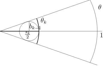
Now, for d(j−, j+)≥ 35sk, we will look at the special configuration given
by Figure 1 when we have rj− =rj+ =bk−1 and the balls are tangent to the
ends of I− and I+. This will give a bound for any possible configuration,
since in any other situation the cone of allowable directions is narrower.
Bj−
Bj+
bk−1
sk
I− I+
Figure 1:
Let us focus on one half of the cone (Figure 2). Let θ be the width of the cone. In this case, we have to look at bθ
k directions that arebk-separated.
Further, we note thatθ = 2θk
sk, where θk is the bold arc at distance sk/2 from
the center of the cone.
θ
1 θk
bk−1
sk
2
Figure 2:
It is clear that θk ∼ bk−1, and therefore the number D of lines in
bk-separated directions with nonempty interesection with Bj− and Bj+ has to satisfy D≤ θ
bk =
2θk
skbk ∼
bk−1 bk
1
sk.
Now we can prove the main result of this section. We have the following
We begin in the same way as in the previous section. Again by Definition 1.8, since E ∈Fh, we have Hhδ(ℓe∩E)>1 for all e∈S for any δ < δE.
Consider the sequence a=
empty fork < k0. Therefore the same holds trivially for Ωkand we have that
S=S
k≥k0Ωk.
The following argument is Remark 1.5 in [18]. Since for each e ∈ Ωk we have (14), we can apply Lemma 4.2 with η = ak
2kak1 toℓe∩Ek. Therefore we
obtain two intervals I−
For this, we will apply Lemma 4.3 for the choice b = {2−k}. The esti-mate we obtain is the number of 2−k-separated directions ei, that intersect simultaneously the balls Bj− and Bj+, given that these balls are separated.
We obtain
where K is the number of elements of the sum. Therefore K & ak
h(2−k).
Consider now a dimension functionh≺has in the hypothesis of the theorem. Then again
To bound this last expression, we use first that there exists α ∈ (0,1) with h(x). xα and therefore h−1(x)& x1
α. We then recall the definition of
the sequence a, ak = ∆0(2−k)−
2α
X
j
h(rj)rj1/2 & X k≥k0
σ(Ωk)1/2∆0(2−k)a
1+2α
2α
k (20)
= X
k≥k0
σ(Ωk)1/2 &1.
The next corollary follows from Theorem 4.4 in the same way as Corollary 3.2 follows from Theorem 3.1.
Corollary 4.5. Let E an F+
α-set. If h is a dimension function satisfying h(x)≥Cxα√xlogθ(1
x) for θ >
1+2α
2α then H
h(E)>0.
Remark 4.6. Note that at the critical value α= 12, we can compare Corol-lary 3.2 and CorolCorol-lary 4.5. The first says that in order to obtain Hh(E)>0
for an F1+ 2
set E it is sufficient to require that the dimension function h
sat-isfies the bound h(x) ≥ Cxlogθ(1x) for θ > 3. On the other hand, the latter says that it is sufficient that h satisfies the bound h(x)≥xlogθ(1
x)for θ >2.
In both cases we prove that an F1+ 2
-set must have Hausdorff dimension at least 1, but Corollary 4.5 gives a better estimate on the logarithmic gap.
5. F0 - sets
In this section we look at a class of very small Furstenberg sets. We will study, roughly speaking, the extremal case of F0-sets and ask ourselves if
inequality (1) can be extended to this class. According to the definition of Fα-sets, this class should be the one formed by sets having a zero dimensional linear set in every direction. We will call a dimension function h “zero di-mensional” if h≺xα for all α >0. Let us introduce the following subclasses of F0:
Fk
0: E ∈F0k if it contains at least k points in every direction.
FN
0 : E ∈F
N
0 if it contains at least countable points in every direction.
Our approach to the problem, using dimension functions, allows us to tackle the problem about the dimensionality of these sets in some cases. We study the case ofFh-sets associated to one particular choice ofh. We will look at the function h(x) = 1
log(1
x)
as a model of “zero dimensional” dimension function. Our next theorem will show that in this case inequality (1) can indeed be extended. The trick here will be to replace the dyadic scale on the radii in Jk with a faster decreasing sequence b={bk}k∈N.
The main difference will be in the estimate of the quantity of lines in bk-separated directions that intersect two balls of level Jk with a fixed distance sk between them. This estimate is given by Lemma 4.3.
We can prove the next theorem, which provide a class of examples of zero simensional Fh-sets.
Theorem 5.1. Let h(x) = 1
log(x1) and let E be an Fh-set. Then dim(E)≥ 1 2.
Proof: Take a nonnegative sequence b which will be determined later. We will apply the splitting Lemma 4.2 as in the previous section. For this, take k0 as in (14) associated to the sequence a={k−2}k∈N. Now, for a given
genericδ-covering ofE withδ <min{δE,2−k0}, we use Lemma 2.2 to obtain
a decomposition S=S
k≥k0Ωk with
k is the partition of the radii associated tob and c >0 is a suitable constant.
We apply the splitting Lemma 4.2 to ℓe∩Ek to obtain two h−1(ck−2
)-j=1 be a bk-separated subset of Ωk. Therefore Mk &Ωk/bk.
We also define, as in Theorem 4.4, Πk :=Jb
By Lemma 4.3, we obtain
and the same calculations as in Theorem 4.4 (inequality (18)) yield
In the last inequality we use that the terms are all nonnegative. The goal now is to take some rapidly decreasing sequence such that the factor b2kβ
bk−1 beats the factor k−4e−ck2
.
Let us take 0< ε < 1−2β2β and consider the hyperdyadic scalebk= 2−(1+ε)k. With this choice, we have
b2kβ bk−1
= 2(1+ε)k−1−(1+ε)k2β
= 2(1+ε)k(1+1ε−2β).
Replacing this in inequality (22) we obtain
X
Finally, since by the positivity of 1+1ε −2β the double exponential in the numerator grows much faster than the denominator, we obtain
2(1+ε)k(1+1ε−2β)
eck2
k4 &1, (23)
Corollary 5.2. Let θ > 0. If E is an Fh-set with h(x) = 1 logθ(1
x)
then
dim(E)≥ 1 2.
Proof: This follows immediately, since in this case the only change will be
h−1(ck−2) = 1
e(ck2)
1
θ,so the double exponential still grows faster and therefore
2(1+ε)k( 11+ε−2β)
e(ck2)1θk4
&1.
This shows that there is a whole class of F0-sets that must be at least 1
2-dimensional.
Now, in the opposite direction, we will show some examples of very small F0-sets. The first observation is that it is possible to construct F0k-sets and
even FN
0-sets with Hausdorff dimension not exceeding 12. This can be done
with some suitable modifications of the construction made in [18], Remark 1.5, (p. 10). There, for each 0 < α ≤ 1, an Fα set is constructed whose dimension is not greater than 12 + 32α. It is straightforward to modify that construction for it to hold even at the endpoint α= 0.
We also include the following example of anF2
0-set G of dimension zero.
It will be constructed using the next result, which is Example 7.8 (p. 104) in [4]. In that example, Falconer constructs sets E, F ⊆ [0,1] with dim(E) = dim(F) = 0 and such that [0,1]⊆E+F.
E× {1}
−F × {0}
x
−y θ
Figure 3:
c = tan(θ), so c∈ [0,1]. By the choice of E and F, we can find x ∈E and y ∈F with c=x+y.
The points (−y,0) and (x,1) belong toGand determine a segment in the direction θ (Figure 3).
6. Acknowledgments
We would like to thank to Michael T. Lacey for fruitful conversations dur-ing his visit to the Department of Mathematics at the University of Buenos Aires.
We also thank the anonymous referee for extremely careful reading of the manuscript and pointing out many subtle improvements which made this paper more readable.
References
[1] Carlos Cabrelli, Franklin Mendivil, Ursula M. Molter, and Ronald Shon-kwiler. On the Hausdorff h-measure of Cantor sets. Pacific J. Math., 217(1):45–59, 2004.
[2] Roy O. Davies. Some remarks on the Kakeya problem. Proc. Cambridge Philos. Soc., 69:417–421, 1971.
[3] M´arton Elekes and Tam´as Keleti. Borel sets which are null or non-σ-finite for every translation invariant measure. Adv. Math., 201(1):102– 115, 2006.
[4] Kenneth Falconer. Fractal geometry. John Wiley & Sons Inc., Hoboken, NJ, second edition, 2003. Mathematical foundations and applications. [5] Ignacio Garcia, Ursula Molter, and Roberto Scotto. Dimension functions
of Cantor sets. Proc. Amer. Math. Soc., 135(10):3151–3161 (electronic), 2007.
[6] Felix Hausdorff. Dimension und ¨außeres Maß. Math. Ann., 79(1-2):157– 179, 1918.
[8] Nets Hawk Katz and Terence Tao. Some connections between Falconer’s distance set conjecture and sets of Furstenburg type.New York J. Math., 7:149–187 (electronic), 2001.
[9] U. Keich. On Lp bounds for Kakeya maximal functions and the Minkowski dimension in R2. Bull. London Math. Soc., 31(2):213–221, 1999.
[10] Themis Mitsis. Norm estimates for the Kakeya maximal function with respect to general measures. Real Anal. Exchange, 27(2):563–572, 2001/02.
[11] L. Olsen. The exact Hausdorff dimension functions of some Cantor sets.
Nonlinearity, 16(3):963–970, 2003.
[12] L. Olsen. On the exact Hausdorff dimension of the set of Liouville numbers. Manuscripta Math., 116(2):157–172, 2005.
[13] L. Olsen and Dave L. Renfro. On the exact Hausdorff dimension of the set of Liouville numbers. II. Manuscripta Math., 119(2):217–224, 2006. [14] C. A. Rogers.Hausdorff measures. Cambridge University Press, London,
1970.
[15] Terence Tao. Finite field analogues of the erdos, falconer, and fursten-burg problems,
http://ftp.math.ucla.edu/∼tao/preprints/expository/finite.dvi.
[16] Terence Tao. From rotating needles to stability of waves: emerging connections between combinatorics, analysis, and PDE. Notices Amer. Math. Soc., 48(3):294–303, 2001.
[17] Thomas Wolff. Decay of circular means of Fourier transforms of mea-sures. Internat. Math. Res. Notices, (10):547–567, 1999.
[18] Thomas Wolff. Recent work connected with the Kakeya problem. In
Prospects in mathematics (Princeton, NJ, 1996), pages 129–162. Amer. Math. Soc., Providence, RI, 1999.
547–567; MR1692851 (2000k:42016)]. J. Anal. Math., 88:35–39, 2002. Dedicated to the memory of Tom Wolff.
![ConsiderFigure 3:and contains two points in every direction G = E × {1} ∪ −F × {0}. This set G has clearly dimension 0, θ ∈ [0; π]](https://thumb-ap.123doks.com/thumbv2/123dok/626803.165948/20.612.213.402.439.596/considerfigure-contains-points-direction-g-set-clearly-dimension.webp)
