Performance Comparison Between Kimura 2-Parameters and Jukes-Cantor Model in Constructing Phylogenetic Tree of Neighbour Joining (NJ)

(1)

PERFORMANCE COMPARISON BETWEEN KIMURA 2-PARAMETERS

AND JUKES-CANTOR MODEL IN CONSTRUCTING PHYLOGENETIC

TREE OF NEIGHBOUR JOINING (NJ)

HENDRA PRASETYA

G14070025

DEPARTMENT OF STATISTICS

FACULTY OF MATHEMATICS AND NATURAL SCIENCES

BOGOR AGRICULTURAL UNIVERSITY

(2)

ABSTRACT

HENDRA PRASETYA. Performance Comparison Between Kimura 2-Parameters and Jukes-Cantor Model in Constructing Phylogenetic Tree of Neighbour Joining (NJ). Advised by ASEP SAEFUDDIN and MULADNO.

Bioinformatics as a recent improvement of knowledge has made an interest for scientist to collect and analyze data to provide the best estimate of the true phylogeny. The objective of this research is to construct and compare the phylogenetic tree of Neighbour Joining (NJ) based on different models (Kimura 2-Parameters and Jukes-Cantor) and to find out which model is more reliable on constructing NJ’s tree. In order to build the tree, reliable set of data is conducted from D-loop mtDNA sequences that is available in Gen Bank. The nucleotide sequences come from

Bison bison (American bison), Bos taurus (European cow such as Shorthorn), Bos indicus (zebu breeds), Bos grunniens mutus (one of subspecies of cow), and Capra hircus (species of goat). The reliability of each models was measured using the Felsentein’s bootstrap method. The whole bootstrap process for each models was repeated 1.000, 5.000, and 10.000 times to detect its reliability. The performance was measured on the basis of the consistency of the topology relationship, the stability of nodes, the consistency of bootstrap confidence level (PB), standard error of distance, change of PB from (1.000-5.000) to (5.000-1.000), computational time, and BIC

score. NJ’s phylogenetic tree with kimura 2-parameters and jukes cantor model have a good node

stability and is also generally successful in representing topological relationships between taxa. The increasing of bootstrap replication number in common will increase the consistency of bootstrap confidence value ( . It means both models have a good reliability. But, when the number of sequences is large and the extent of sequence divergence is low, it is generally difficult to construct the tree by any models. In conclusion, Kimura 2-Parameters has a better performance than Jukes-Cantor.

(3)

PERFORMANCE COMPARISON BETWEEN KIMURA 2-PARAMETERS

AND JUKES-CANTOR MODEL IN CONSTRUCTING PHYLOGENETIC

TREE OF NEIGHBOUR JOINING (NJ)

HENDRA PRASETYA

G14070025

Research Report

to complete the requirement for graduation of Bachelor Degree in Statistics

at Department of Statistics

Faculty of Mathematics and Natural Sciences

Bogor Agricultural University

DEPARTMENT OF STATISTICS

FACULTY OF MATHEMATICS AND NATURAL SCIENCES

BOGOR AGRICULTURAL UNIVERSITY

(4)

Title : Performance Comparison Between Kimura 2-Parameters and Jukes-Cantor Model in Constructing Phylogenetic Tree of Neighbour Joining (NJ)

Author : Hendra Prasetya

NIM : G14070025

Approved by:

Advisor I, Advisor II,

Dr. Ir. Asep Saefuddin, M.Sc Prof. Dr. Ir. Muladno, MSA

NIP. 195703161981031004 NIP. 196108241986031001

Acknowledged:

Head of Department of Statistics

Faculty of Mathematics and Natural Sciences IPB

Dr. Ir. Hari Wijayanto, M. Si NIP. 1965042111990021001

(5)

BIOGRAPHY

Hendra Prasetya was born in Banyumas, on September 25th, 1989, as the first son of Muhammad Mahrudin and Aminah. He has a younger brother.

The author started his first education in Sekolah Dasar Negeri (SDN) Rawaheng 03 in 1995 and finished it in 2001. His next study was in Sekolah Lanjutan Tingkat Pertama Negeri (SLTPN) 01 Wangon from 2001-2004 and then continued to Sekolah Menengah Atas Negeri (SMAN) 01 Jatilawang until 2007. The writer had been received as a student of Bogor Agricultural Univeristy (IPB) after passing USMI, exactly in Department of Statistics. During February-March 2011, he had an opportunity to join an internship program in Pusat Data Informasi Ketenagakerjaan (Pusdatinaker), Balitfo, Kementerian Ketenagakerjaan dan Transmigrasi (Kemenakertrans) RI.

During his study in IPB, he was active in some collage organizations, for example as Chief of Community Development Department - FORCES (Forum for Scientific Study) (2010); Secretary of Social Responsibility Division - LDK Al Hurriyyah (2007-2008); Staff of Syiar Departement - LDK Al

Hurriyyah (2008-2009); Staff of Education Ministry - BEM KM IPB “Generasi Inspirasi” (2010); Staff of

Badan for Palestine (BFP) - KAMMI Komsat IPB / Izzudin Al Qassam (2008-2009); Comission II of

Student Advisory Board – Faculty of Mathematics and Natural Sciences (2009); Head of MAPRES

School - Forum Silaturrahim Lembaga Dakwah Kampus IPB / FSLDKI (2010); and Supporter of Greenpeace South East Asia.

Furthermore, the writer was also known as an active student in many kinds of scientific events, in IPB, national, and international level. Some achievements have ever been carved are:

1. Presenter of International Conference of Aceh Development International Conference in Universiti Kebangsaan Malaysia, Malaysia, 2011,

2. Proceeding Paper of International Journal of AISC, Taiwan, 2011,

3. Selected Scientific Paper to be presented in International Conference of Applied Energy, Italy, 2011,

4. Selected Scientific Paper to be presented in Education Without Border, Saudi Arabia, 2011,

5. Selected Scientific Paper to be presented in AMSTEC, Japan, 2011,

6. The 2nd Winner of Mahasiswa Berprestasi (MAPRES) of IPB, 2010,

7. The 1st Winner of Mahasiswa Berprestasi (MAPRES) of FMIPA, 2010,

8. The 1st Winner of Mahasiswa Berprestasi (MAPRES) of Department of Statistics, 2010,

9. The 1st Winner of National Scientific Paper and Bussiness Plan Competition, “Make and Sell

Competition (MSC)”, in Institut Teknologi Sepuluh November (ITS), Surabaya, 2009,

10.The 1st Winner of HIBAH MITI (Masyarakat Ilmuan dan Teknolog Indonesia) for Jakarta-Jabar-Banten (Jabaja) Regional, as Assocation with Ministry of Research and Technology (Kemenristek), Republic of Indonesia, 2010,

11.The 1st Winner of The Most Outstanding Student in IPB’s Dedication for Education (IDEA), 2010, 12.The 3rd Winner of National Statistical Scientific Paper Competition, Student Level, in Universitas

Gajah Mada (UGM), Jogjakarta, 2008,

13.The 3rd Winner of National Scientific Paper Writing Competition of Cultural Journal, in Universitas Indonesia (UI), Depok, 2009,

14.The 4th Winner of National Scientific Paper Competition, “Lomba Karya Cipta Mahasiswa (LKCM)”,

in IPB, Bogor, 2009,

15.The Finalist of National Scientific Paper and Bussiness Plan Competition, “ITB Entrepreneurship

Challenge (IEC)”, Institut Teknologi Bandung (ITB), Bandung, 2009,

16.The Finalist of PIMNAS XXII, Field of Non PKM, “Kompetisi Karya Tulis Al Qur’an (KKTA)”, Universitas Brawijaya (UB), Malang, 2009,

17.The Receiver of International Scholarship: Korean Exchange Bank Scholarship, 2010,

18.The Receiver of International Scholarship: Belgrade Summer School Partial Scholarship, 2009,

19.The IPB’s Exhibition Team in PIMNAS (Pekan Ilmiah Mahasiswa Nasional), Universitas Brawijaya (UB), Malang, 2009,

20.IPB’s Delegation in Indonesia Leadership Camp (ILC), Universitas Indonesia (UI), 2010, 21.IPB’s Delegation in Sampoerna Best Student Visit (SBSV), PT Sampoerna Tbk, Surabaya, 2010,

22.A Fund Award from Dikti in Program Kreativitas Mahasiswa (PKM): 1 PKM Artikel Ilmiah (2009), 1

PKM Penelitian (2009), 1 PKM Kewirausahaan (Tahun 2010), 2 PKM Artikel Ilmiah (2010), 1 PKM Penelitian (2009),

23.The Finalist of Lomba Karya Tulis Ilmiah Al Qur’an (LKTIA) MTQ IPB, 2011,

24.The Most Active Author of Sanggar Tinta Cahaya (STC), KAMDA Bogor, November 2010,

(6)

ACKNOWLEDGEMENTS

Syukur alhamdulillah, many grateful thanks are only to Allah SWT Who always gives me a mercy, a blessing, an endless love, a capability, and a big fervency, especially in finishing my

researh entitles “Performance Comparison between Kimura 2-Parameters and Jukes-Cantor Model

in Constructing Phylogenetic Tree of Neighbour Joining (NJ)”. This scientific paper is composed

to complete the graduation requirement of Bachelor Degree in Statistics at Department of Statistics, Faculty of Mathematics and Natural Sciences, Bogor Agricultural University.

I am really aware and have to admit that my research could not be completed without any helps and supports from some stakeholders. A million appreciations are presented for their ideas, correction, and improvement during the process. Therefore, I would like to extend gratitude very much to all people have helped me in finishing this research, especially to:

1. Dr. Ir. Asep Saefuddin, M.Sc dan Prof. Dr. Ir. Muladno, MSA, as my advisors who had given a

really expert guidances, motivations, and useful suggestions,

2. My beloved parents and younger brother (Aditya Khoirul Ramadhan Prasetya) for a do’a and a

sincere affection,

3. My brothers and sisters in arms: The Ilmy Team of Ceria 1432 H, Al Banna Family, BM Family, Statistics Family 44, Abi Ary Santoso, Abi Muhammad Irfan, Rizki Alkindi, Ahmad DJ Pakaya, Aris Yaman, Tia Fitria A., Fitrie Indrianie, and mujahid-mujahiddah of tarbiyyah

IPB who always gives a lot of inspirations about the meaning of both forshoot real fighting and the bauty of ukhuwatul islamiyah,

4. All family of statistics and stakeholders who had helped and supported me in completing the

research and finishing this paper.

For the last, I would like to ask permission for some guiltiness in case of writing or on going of researh process. A wise correction and evaluation are also really hoped from the readers due to a better future knowledge. Finally, I wish that this little work could be useful for all. Thank you.

Bogor, July 2011

(7)

CONTENT

Page

LIST OF TABLE... ix

LIST OF FIGURE... ix

LIST OF APPENDIX... x

INTRODUCTION 1 Background... 1

Objectives... 1

LITERATURE REVIEW... 1

Phylogenetic Tree... 1

Mitochondrion DNA... 2

Neighbour Joining Method... 2

Kimura 2-Parameters Model... 2

Jukes-Cantor Model... 3

Bootstrap... 3

METHODOLOGY... 4

Data Sources... 4

Methods... 4

RESULT AND DISCUSSION... 5

Molecular Data Exploratiom... 5

Distance Matrix... 6

Performance of NJ’s Phylogenetic Tree with Kimura 2-Parameters Model... 6

Performance of NJ’s Phylogenetic Tree with Jukes-Cantor Model... 7

Performance Comparison Both Models in Constructing NJ’s Tree... 8

CONCLUSION... 10

RECOMMENDATION... 10

REFERENCES... 10

(8)

LIST OF TABLE

Page

Table 1 The Nucleotide Substitution Composition of Kimura 2-Parameters... 3

Table 2 The Nucleotide Substitution Composition of Jukes-Cantor... 3

Table 3 List of Organisms, Accession Number, and Sequence Length of D-loop... mtDNA 4 Table 4 The Average of Nucleotide Composition... 5

Table 5 The Proportion of Nucleotides Pairs... 6

Table 6 Overall Mean and Standard Error for Each Group... 6

Table 7 Missedclassification Between Taxa in NJ’s Tree for Both Models... 8

LIST OF FIGURE

Page Figure 1 Evolutionary Tree Components... 1

Figure 2 Example of Star Tree with Five Taxon... 2

Figure 3 Example of Nodes Neighbours... 2

Figure 4 Phylogenetic Tree with Kimura 2-Parameters Model of Group E... 7

Figure 5 A Comparison of Stable Nodes Percentage for Each Group... 9

(9)

LIST OF APPENDIX

Appendix 1. Spesification of D-loop mtDNA Sequences for All Organisms

Appendix 2. The Proportion of The Four Nucleotides Composition to All Organisms

Appendix 3. Comparison of Number and Proportion of Stable Nodes for Kimura 2-Parameters

and Jukes-Cantor for All Groups and Each Bootstrap Replications

Appendix 4. The Consistency Change of Bootstrap Confidence Value (PB) from (1.000-5.000) to

(5.000-10.000)

Appendix 5. a. Some Statistics and Informations of The Built Cases Group A-D

b. Some Statistics and Information of The Built Cases Group E-G

Appendix 6. Bootstrap Consensus Tree of Group A with Kimura 2-Parameters Model,

Respectively for 1.000 (a), 5.000 (b), 10.000 (c) Repeated Times

Appendix 7. Bootstrap Consensus Tree of Group B with Kimura 2-Parameters Model,

Appendix 8. Bootstrap Consensus Tree of Group C with Kimura 2-Parameters Model,

Appendix 9. Bootstrap Consensus Tree of Group D with Kimura 2-Parameters Model,

Appendix 10.Bootstrap Consensus Tree of Group E with Kimura 2-Parameters Model,

Appendix 11.Bootstrap Consensus Tree of Group F with Kimura 2-Parameters Model,

Appendix 12.Bootstrap Consensus Tree of Group G with Kimura 2-Parameters Model,

Appendix 13.Bootstrap Consensus Tree of Group A with Jukes-Cantor Model, Respectively for 1.000 (a), 5.000 (b), 10.000 (c) Repeated Times

Appendix 14.Bootstrap Consensus Tree of Group B with Jukes-Cantor Model, Respectively for 1.000 (a), 5.000 (b), 10.000 (c) Repeated Times

Appendix 15.Bootstrap Consensus Tree of Group C with Jukes-Cantor Model, Respectively for 1.000 (a), 5.000 (b), 10.000 (c) Repeated Times

Appendix 16.Bootstrap Consensus Tree of Group D with Jukes-Cantor Model, Respectively for 1.000 (a), 5.000 (b), 10.000 (c) Repeated Times

Appendix 17.Bootstrap Consensus Tree of Group E with Jukes-Cantor Model, Respectively for 1.000 (a), 5.000 (b), 10.000 (c) Repeated Times

Appendix 18.Bootstrap Consensus Tree of Group F with Jukes-Cantor Model, Respectively for 1.000 (a), 5.000 (b), 10.000 (c) Repeated Times

Appendix 19.Bootstrap Consensus Tree of Group G with Jukes-Cantor Model, Respectively for 1.000 (a), 5.000 (b), 10.000 (c) Repeated Times

Appendix 20.Consistency Comparison among NJ’s Tree with Kimura 2-Paramaters and

Jukes-Cantor Conducted to All Built Cases

Appendix 21.Comparison of Computational Time among Both Models and Cases

Appendix 22.Value of BIC of Each Group for Both Models

Appendix 23.Substution (Transition and Tranversion) Rate of Kimura 2-Parameters and Jukes-Cantor

Appendix 24.Mean (black font colour) and Standard Error (blue font colour) of Distance Matrix

of Group E with Kimura 2-Parameters Model

Appendix 25.Mean (black font colour) and Standard Error (blue font colour) of Distance Matrix

of Group E with Jukes-Cantor Model

(10)

Appendix 26.Original Tree of NJ’s Tree with Kimura 2-Parameters for Group A (a), Group B (b), Group C (c), Group D (d), Group E (e), Group F (f), & Group G (g)

Appendix 27.Original Tree of NJ’s Tree with Jukes-Cantor for Group A (a), Group B (b), Group

C (c), Group D (d), Group E (e), Group F (f), and Group G (g)

Appendix 28.Evolutionary Distance among Species of Group B with Jukes-Cantor (J-C) and

Kimura 2-Parameters (K 2-P) Model

Appendix 29.Mean of Distance Matrix for All Organisms with Kimura 2-Parameters Model

Appendix 30.Mean of Distance Matrix for All Organisms with Jukes-Cantor Model

(11)

1

INTRODUCTION

Background

Bioinformatics as a recent improvement of knowledge has made an interest for scientist to collect and analyze data to provide the best estimate of the true phylogeny. Phylogenetics construction methods attempt to find the evolutionary history of a given set of species (Elfaizi et al. 2004). A phylogenetic or

evolutionary tree elucidates functional

relationship within living cells. It is

constructed by using all kinds from molecular data in the form of individual protein or nucleic acid sequences.

Nowadays there are three major methods for performing a phylogenetic analysis: Distance-Based method (UPGMA, ME, and NJ), Maximum Parsimony, and Maximum Likelihood (Otu et al. 2003). If spesifically we would like to have the information about the evolutionary distance among sequences, a distance-based method should be used. A previous research had shown that NJ (Neighbour Joining) method is better than ME

(Minimum Evolution) and UPGMA

(Unweighted Pair-Group Method using

Arithmetic Average) (Putri 2010). The Neighbour Joining method is a greedy algorithm because it has high accuracy on measuring a distance between two mtDNA sequences.

Then, NJ method itself can be used to construct evolutionary tree by some models, such as Kimura 2-Parameters and Jukes-Cantor. Each model has its own formulation to calculate the distance matrix, so the resulted phylogenetic tree will tend to have different performance. Therefore, one of the challenges is to choose a model of DNA substitution that excellently describes the data in hand by statistical approach. Generally speaking, the aim is to pick a model that adequately explains the data (in this case an alignment of DNA sequences).

With the increasing emphasis on tree construction, questions arose as to how confident one should be in a given phylogenetic tree and how support for phylogenetic tree should be measured. Felsenstein (1985, refers to Soltis & Soltis 2003) formally proposed bootstrapping as a method for obtaining confidence limits on phylogenies.

In this paper, we used a whole D-loop mtDNA sequences. Its variations have been widely applied in population genetics study of

creatures such as animals due to the maternal inheritance and high substitutions of this organelle genome. At last, in order to compare the performance of NJ’s tree for each model, D-loop mtDNA sequences of five different

species were used to compare the

performance. They were Bison bison, Bos

taurus, Bos indicus, Bos grunniens mutus, and

Capra hircus. The performance was measured using some aspects: the representing of topologies relationship, computational times, consistency, the node stability, and some criterias. Otherwise, the consistency was measured using bootstrap procedure.

Objectives

The objectives of this research are:

1. to construct and compare the phylogenetic

tree of NJ based on different models (Kimura 2-Parameters and Jukes-Cantor), 2. to find out which model is more reliable

on constructing NJ’s tree in which case.

LITERATURE REVIEW

Phylogenetic tree

Phylogenetics describes the relationship between genes, proteins, or species. In phylogenics, the objects are being assumed to be evolutionary related. The evolutionary or phylogenetic tree is used to show the evolutionary relationship among organisms. To build the correct evolutionary tree, we also need a correct and proper data. The correct and proper data could be (Li 2001): (1) taxa: the groups of organisms that we are interested to know the evolutionary relationship, (2) characters: a list of organism phenotype characteristics and some groups of organisms that have different phenotype characteristics. The components of the evolutionary tree are mentioned in Figure 1.

Figure1 Phylogenetic Tree Components

There are numerous methods for

constructing phylogenetic trees from

(12)

2

taxa, and a phylogenetic tree is constructed by considering the relationships among these distance values.

Mitochondrion DNA

Mitochondrion DNA (mtDNA) is the

DNA constituting an organelle called

mitochondria, structures within cells that convert the energy from food into a form which cells can use. The organelle is located in the cytoplasm of the cell. D-loop occurs in the main non-coding area of the mtDNA molecule, a segment called the control region. The region has proven to be useful for the

study of the evolutionary history of

vertebrates (Larizza A et al. 2002). In constructing phylogenetic tree, we use part of D-loop mtDNA sequences available in gene bank for all organisms.

Neighbour Joining Method

This method (Saitou et al. 1987) is a simplified version of the minimum evolution (ME) method. Construction of a tree by the NJ

method begins with a ‘star’ tree, which is produced under the assumption that there is no clustering of taxa. We then estimate the

branch lengths of the ‘star’ tree and compute

the sum of all branches ( ). This sum should

be greater than the sum for the final NJ’s tree

( ).

∑

⁄

where is the total number of sequence used,

is the branch length estimate between

nodes and , and ∑ .

In practice, since we do not know which pairs of taxa are true neighbours, we consider all pairs of taxa as a potential pair of taxa are true. We then choose the taxa and that show the smallest value. This procedure is repeated until the final tree is produced.

where ∑ and ∑ .

Once the smallest determined, we can

create a new node ( ) that connects taxa and

. The branch lengths ( ) is given by the following formula:

,

.

The next following step is to compute the distance between the new node ( ) and the remaining taxa.

A complete algorithm is given below: 1. We start off with a star tree (Figure 2).

Figure 2 Example of Star Tree with Five Taxon

2. We define some kind of distance

parameter between our nodes (1 through 5) and enter this parameter into a distance matrix (see following paragraphs). The columns and rows of the matrix represent nodes and the value i and j of the matrix represent the distance between node i and node j. Note that the matrix is symmetric and the diagonal is irrelevant. Therefore, only the top half (or lower half) are enough.

3. We pick the two nodes with the lowest value in the matrix defined in step 2 as neighbours. For example, assuming nodes 1 and 2 are the nearest, we define them as neighbours (Figure 3).

Figure 3 Example of Nodes Neighbours

4. The new node we have added as node X.

5. We now define the distance between node

X and the rest of the nodes, and enter these distances into our distance matrix. We remove nodes 1 and 2 from our distance matrix.

6. We compute the branch lengths for the branches that have been joined (for figure 2(b), these are branches 1-X and 2-X) . 7. We repeat the process from stage 2 – once

again we look for the 2 nearest nodes, and so on.

Kimura 2-Parameters Model

(13)

3

symbolized as α, whereas the rate of

transversion is as β (Kimura 1980). The Table 1 shows the composition of nucleotide substitution.

Table 1 The Nucleotide Substitution Composition of Kimura 2-Parameters

A T C G

A - β β α

T β - α β

C β α - β

G α β β -

The matrix distance between two mtDNA sequences are computed based on the number of nucleotide substitutions (transition and transversion) per site (d), the number of transitional substitutions per site (s), and the number of transversional substitutions per site (v). We can also compute the value of transition/transversions ratio (R).

Formulas for computing these quantities are as follows:

⁄ ⁄ ,

⁄ , R = s/v,

where P and Q are the proportion of sites with transitional and transversional differences respectively, and

,

.

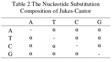
Jukes-Cantor Model

In the Jukes-Cantor model, the rate of nucleotide substitution is the same for all pairs of four nucleotides A, T, C, and G. As is shown below, the multiple hit correction equation for this model produces a maximum likelihood estimate of the number of

nucleotide substitutions between two

sequences. It assumes an equality of

substitution rates among sites, equal

nucleotide frequencies, and it does not correct for higher rate of transitional substitutions as compared to transversional substitutions. The rate of transition is symbolized as α (Jukes et

al. 1969). The Table 2 shows the composition

of nucleotide substitution. Formulas for computing the distance between two mtDNA sequences are:

⁄ ⁄

where p is the proportion of sites with different nucleotides.

Table 2 The Nucleotide Substitution Composition of Jukes-Cantor

A T C G

A - α α α

T α - α α

C α α - α

G α α α -

Bootstrap

One of the most commonly used tests of the reliability of an inferred tree is Felsentein’s bootstrap test (refers to Soltis & Soltis 2003). A bootstrap data matrix x* is formed by randomly selecting n columns from the original matrix x. Then the original tree-building algorithm is applied to x*, giving a bootstrap tree as :

̂ ̂

Then, the proportions of bootstrap trees

‘agreeing’ with the original tree are

calculated. These proportions are the

bootstrap confidence values (PB). When the bootstrap resampled data set is obtained, an estimate of distance is computed for each sequence. This procedure is repeated B times.

One assumption often made for the

bootstrap is that all sites evolve

independently. This assumption of course does not hold in the present case. However, if the number of sites examined is large (n >100) as in the present case, the effect of violation of the assumption is not important because most sites with different evolutionary rates will be represented in each bootstrap sample.

The result of bootstrap method gives information about the number of nodes

formed from B replication of bootstrap.

Boostrapping measures how consistently the data support given taxon bipartitions (Hedges 1992). This is not a test of how accurate your tree is; it only gives information about the stability of the tree topology (the branching order), and it helps assess whether the sequence data is adequate to validate the topology (Berry et al. 1996).

(14)

4

METHODOLOGY

Data Sources

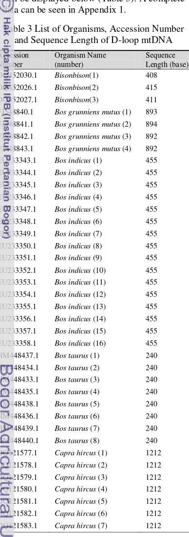
For this research, the dataset of D-loop mtDNA sequences was obtained from Gen Bank (www.ncbi.nlm.nih.gov) for free. The data was accessed on March, 20th 2011. The nucleotide sequences come from some organisms as taxon. List of organisms, sequence length (base), and accession number will be displayed below (Table 3). A complete data can be seen in Appendix 1.

Table 3 List of Organisms, Accession Number and Sequence Length of D-loop mtDNA

Accession Number

Organism Name (number)

Sequence Length (base) DQ452030.1 Bisonbison(1) 408 DQ452026.1 Bisonbison(2) 415 DQ452027.1 Bisonbison(3) 411 FJ548840.1 Bos grunniens mutus (1) 893 FJ548841.1 Bos grunniens mutus (2) 894 FJ548842.1 Bos grunniens mutus (3) 892 FJ548843.1 Bos grunniens mutus (4) 892 EU233343.1 Bos indicus (1) 455 EU233344.1 Bos indicus (2) 455 EU233345.1 Bos indicus (3) 455 EU233346.1 Bos indicus (4) 455 EU233347.1 Bos indicus (5) 455 EU233348.1 Bos indicus (6) 455 EU233349.1 Bos indicus (7) 455 EU233350.1 Bos indicus (8) 455 EU233351.1 Bos indicus (9) 455 EU233352.1 Bos indicus (10) 455 EU233353.1 Bos indicus (11) 455 EU233354.1 Bos indicus (12) 455 EU233355.1 Bos indicus (13) 455 EU233356.1 Bos indicus (14) 455 EU233357.1 Bos indicus (15) 455 EU233358.1 Bos indicus (16) 455 HM448437.1 Bos taurus (1) 240 HM448434.1 Bos taurus (2) 240 HM448433.1 Bos taurus (3) 240 HM448435.1 Bos taurus (4) 240 HM448438.1 Bos taurus (5) 240 HM448436.1 Bos taurus (6) 240 HM448439.1 Bos taurus (7) 240 HM448440.1 Bos taurus (8) 240 DQ121577.1 Capra hircus (1) 1212 DQ121578.1 Capra hircus (2) 1212 DQ121579.1 Capra hircus (3) 1212 DQ121580.1 Capra hircus (4) 1212 DQ121581.1 Capra hircus (5) 1212 DQ121582.1 Capra hircus (6) 1212 DQ121583.1 Capra hircus (7) 1212

Bison bison is well known as American

bison. On the other hand, Bos grunniens

mutus is one of subspecies of cow and Capra hircus is a species of goat. While Bos taurus

is European cow such as Shorthorn and Jersey, Bos indicus is a zebu breeds such as Brahman.

Methods

The procedures to conduct this research are:

1. Access the complete D-loop mtDNA

sequence which consists of five spesies, from Gen Bank. Then, copy and paste it into notepad, and save it in format .txt. The available data sets were:

a. Bison bison [3] b. Bos taurus [8] c. Bos indicus [16] d. Bos grunniens mutus [4] e. Capra hircus [7]

The number in parenthesis shows the amount of sequences.

2. Build the cases by making some groups of

taxon which are:

a. Group A consists of: Bison bison [3],

Bos taurus [8], Bos indicus [16], Bos grunniens mutus [4], Capra hircus [7].

b. Group B consists of: Bison bison [3],

Bos taurus [3], Bos indicus [3], Bos grunniens mutus [3], Capra hircus [3]. c. Group C consists of: Bison bison [3],

Bos taurus [1], Bos indicus [1], Bos grunniens mutus [1], Capra hircus [1]. d. Group D consists of: Bison bison [1],

Bos taurus [8], Bos indicus [1], Bos grunniens mutus [1], Capra hircus [1].

e. Group E consists of: Bison bison [1], Bos taurus [1], Bos indicus[16], Bos grunniens mutus [1], Capra hircus [1]. f. Group F consists of: Bison bison [1],

Bos taurus [1], Bos indicus [1], Bos grunniens mutus [4], Capra hircus [1]. g. Group G consists of: Bison bison [1],

Bos taurus [1], Bos indicus [1], Bos grunniens mutus [1], Capra hircus [7]. Numbers in the brackets show the amount of sequences that was used to build the cases. The sample of species used in a group was selected randomly from available sequences.

3. Convert the .txt file of each taxon group

into format fasta by using ClustalX2

software.

4. Align all data sets by using MEGA 5

(15)

5

number of the D-loop mtDNA sequence here is around 1.223 base-pairs length (before the gaps edited). Both insertions and deletions introduce gaps in the DNA sequence alignment due to the alignment procedure, so we need to delete all gaps in the data sets. The total length of the D-loop mtDNA sequence here already been reduced to 395,46 base-pairs length. 5. Do the molecular data exploration, such

as: nucleotide composition, the transition/ transversion rate ratios, nucleotide pair frequency, and the overall transition/ transversion bias (R). The aim is to know the characteristics of data.

6. Construct the original phylogenetic tree of NJ with Kimura 2-Parameters and Jukes-Cantor model. The mean and its standard errors of estimated distance for all groups were also counted.

7. Then, compare the perfomance of each

model by checking the reliability of each model using the bootstrap procedure with 1.000, 5.000, and 10.000 repeated times. In addition, we also compute some values such as missedclassification to see the consistency of the topology relationship,

proportion of stable nodes (%),

consistency of bootstrap confident value (PB), change of PB from (1.000-5.000) to (5.000-1.000), computational time, and BIC score to see the performance each method.

Note that to conduct the alignment, tree construction, and analysis (point 4-7), we use the open-sourced software, MEGA 5.

RESULT AND DISCUSSION

Molecular Data Exploration

A sequnces of mtDNA for each species in this research have a different sequence lengths. The length of sequence points out the number of nucleotide for a particular sequence. In this case, organism with the longest length is Capra hircus number 1-7 (1.212 nucleotides). Otherwise, organism with the shortest length is Bos taurus number 1-8 (240 nucleotides).

The average of sequence length of each group after alignment and gap deletion could be taken a look in Tabel 5(a) and 5(b). Total nucleotides in Group A is as much as 396 with a focus of analysis is the topological relationships of all species. Group B, C, E, F, and G, respectively, have the number of nucleotides of (423), (371), (261), (423),

(540), and (748). Each group is a case that has been built to see the topology or taxa relationship: all species (A), captured three individuals (B), the species of Bison bison

(C), the species of Bos taurus (D), the species of Bos indicus (E), the species of Bos grunniens mutus (F), and the species of Capra hircus (G).

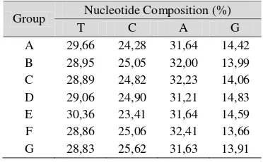
The proportion of nucleotide is a relative frequency of four nucleotides (T, C, A, G) which can be calculated for one or all of the chain in percentage unit. Overall, the proportion of the four nucleotides of each organism is not much different (Appendix 2). To the average of nucleotide number from the mtDNA chains within each group can be seen in Table 4. The proportion value of nucleotides for each group shows the same composition where the highest proportion is in the nucleotide A. Then, it is followed by nucleotide T and C. The lowest proportion is owned by nucleotide G.

Table 4 The Average of Nucleotide Composition

Group Nucleotide Composition (%)

T C A G

A 29,66 24,28 31,64 14,42 B 28,95 25,05 32,00 13,99 C 28,89 24,82 32,23 14,06 D 29,06 24,90 31,21 14,83 E 30,36 23,41 31,64 14,59 F 28,86 25,06 32,41 13,66 G 28,83 25,62 31,63 13,91

The frequency of nucleotide pairs

describes the number of nucleotides which are identical and have the substitution of a comparison chain. In this analysis there are four indicators which are identical pairs (ii), transitional pairs (si), transversional pairs (sv), and the ratio of transition to transversion (R).

(16)

6

In common the si value is always higher than the sv value. The si value represents the average of transition appears, while the sv value represents the avarage of tranversion apperas in the sequences compared. A rasio from transition to tranversion is given as the R value. The R value for Group A, B, D, E, F, and G successively is as many as (1,68), (1,58), (1,85), (3,19), (2,66), (2,08), and (1,82). In other word, it can be stated that the tranversion happens in Group A, B, C, D, E, F, and G is (0,59), (0,63), (0,54), (0,31), (0,38), (0,48), and (0,55) times more of the transition frequency. More complete data has been performed in Table 5.

Table 5 The Proportion of Nucleotides Pairs

Group % ii R % si % sv

A 88,76 1,68 7,08 4,30

B 85,01 1,58 9,23 5,92

C 84,53 1,85 9,99 5,40

D 90,99 3,19 6,91 2,30

E 95,70 2,66 3,08 1,18

F 87,94 2,08 8,16 3,90

G 90,71 1,82 6,02 3,34

avg 89,09 2,13 7,21 3,76

Distance Matrix

In Table 6, we can see the overall mean of estimated distance for all groups. The standard error of both Kimura 2-Parameters model and Jukes-Cantor are relatively small and almost same for each group. Efron B et al. (1996) mentioned that the S.E of 0,052 in their research precisely could be stated as a small value. The standard error is computed using bootstrap procedure with 1.000 repeated times or replications.

Table 6 Overall Mean and Standard Error for Each Group

Group Mean S.E

K 2-P J-K K 2-P J-K

A 0,121 0,118 0,014 0,014

B 0,140 0,136 0,017 0,016

C 0,128 0,125 0,016 0,015

D 0,088 0,085 0,012 0,011

E 0,056 0,054 0,007 0,007

F 0,136 0,132 0,018 0,016

G 0,137 0,134 0,017 0,017

This result shows that the two models are good enough to be used in constructing the phylogenetic tree. However, Kimura 2-Parameters model always has higher standard error than Jukes-Cantor for all groups. For

more detail information of distance matrix for both models, we can take a look into tables in Appendix 29 and Appendix 30.

Performance of NJ’s Phylogenetic Tree with Kimura 2-Parameters Model

The result of original NJ’s tree for each groups are displayed in Appendix 26, while bootstrap NJ’s pylogenetics tree for each groups and each replications are displayed in

Appendix 6 to Appendix 12. NJ’s

phylogenetic tree with Kimura 2-Parameters model is generally successful in representing topological relationships between taxa. They are only Group A, B, C, and D which have a missedclassification in the original tree. However, the missedclassification rate are really small {2,63% (A), 6,67% (B), 14,29% (C), 8,33% (D)}. For those four groups, the taxa of Bison bison 2 is classified wrongly. Based on the taxonomy knowledge, it should be in a cluster of Bison bison. In the phylogenetic tree, it shows an information that

Bison bison 2 is always closer to group of Bos taurus.

In addition, NJ’s tree with this model has a

consistent topological relationship among taxa. It is indicated with a clade position which is identic in phylogenetic tree in the bootstrap phylogenetic tree of 1.000, 5.000, and 10.000 replications. There are five groups from seven groups that have a stable phylogenetic tree in describing the topological relationships for all taxa. They are Group B, C, D, E, and F. Conversely, Group A and G show varying results (inconsistent) or there are topologies changing the sequences.

In Group A some of consistent topological relationships are only clade (Bison bison

1-Bison bion 3); taxon (Bos taurus 3-(Bos taurus 6-(Bos taurus 1-(Bison bison 2-(Bos taurus 7-(Bos taurus 4-(Bos taurus 5))))); taxon Bos indicus 3-Bos indicus 7-Bos indicus

1-Bos indicus 2; taxon (((Bos indicus 9-Bos indicus 11)-Bos indicus 9)-Bos indicus 9); and taxon (Bos grunniens mutus 2-(Bos grunniens mutus 3-(Bos grunniens mutus 4))). In Group G some consistent topological relationship is only valid in describing the taxon (((Bison bison 2-Bos taurus 1)-Bos indicus 14)-Bos grunniens mutus 4).

This NJ’s tree has a good node stability. A stable node has a bootstrap confidence value

( at least 0.5 or 50% (Lesvian 2010).

(17)

7

stability, namely Group E (Figure 4) as many as 35,29% for 1.000 replications of bootstrap and 29,41% for the replication of 5.000 and 10.000. While the six other groups have a proportion greater than or equal to 50%. This

can happen because in general the

evolutionary distance in Group E, especially

between organisms Bos indicus, are very

small and close to 0.

Figure 4 Phylogenetic Tree with Kimura 2-Parameters Model for Group E

The bootstrap confidence value ( for

Kimura 2-Parameters model is not always stable or always experience a change for every increase of bootstrap replications. Sometimes it went up and down. In addition, a changes in the consistency of bootstrap confidence value

( from (1.000-5.000) to (5.000-10.000)

also decreases, but only happened in Group B (from 91,67% to 66,67%), C (from 75% to 50%), and G (from 62,5% to 12,5%) as we could see in Appendix 4.

Nevertheless, the consistency of bootstrap

confidence value ( , both on changes in the

bootstrap replications of 1.000-5.000 and

5.000-1.000 show the proportion of

consistency is more than 50% (Appendix 5(a) and 5(b)). Moreover, the percentage of consistency change for bootstrap confidence

value ( moves up when the repeated times

raises from 1.000-5.000 to 5.000-10.000. It means that when the variation among the used sequence is high, the increase of bootstrap repeated times will increase the percentage of consistency change for bootstrap confidence value ( . Therefore, the reability of NJ’s

tree with Kimura 2-Parameters model

averagely is fine.

Performance of NJ’s Phylogenetic Tree with Jukes-Cantor Model

The result of original NJ’s tree for each

Groups are displayed in Appendix 27, while bootstrap NJ’s pylogenetics tree for each groups and each replications are displayed in Appendix 13 to Appendix 19. As with Kimura

2-Parameters, NJ’s phylogenetic tree with

Jukes-Cantor model is also generally

successful in representing topological

relationships between taxa. They are only Group A, B, C, and D which have a missedclassification in the original tree. However, the missedclassification rate are really small {2,63% (A), 6,67% (B), 14,29% (C), 8,33% (D)}. For those four groups, the taxa of Bison bison 2 is classified wrongly. Based on the taxonomy knowledge, it should be in a cluster of Bison bison. In the phylogenetic tree, it shows an information that

Bison bison 2 is always closer to group of Bos taurus.

NJ’s phylogenetic tree with Jukes-Cantor model has a high nodes stability too because

the value of bootstrap confidence value ( is

more than 50% in seven groups, namely A, B, C, D, F, and G. The percentage of stable nodes for each group can be seen in Appendix 3. Only Group E (same with Figure 2) has a lower proportion of stable nodes, that is equal to 35,29% for 1.000 times of bootstrap replication and 29,41% for 5.000 and 10.000 replication. In general it is due to the evolutionary distances that develops in Group E, in particular among organisms Bos indicus, are very small and close to 0.

In addition, NJ’s tree with Jukes-Cantor model is also generally successful in representing topological relationships between taxa. A consistent topological relationship among taxa is indicated with a clade position which is identic in phylogenetic tree in the bootstrap phylogenetic tree of 1.000, 5.000, and 10.000 replications. There are only three from seven groups that have a stable phylogenetic tree in describing the topological relationships for all taxa. They are Group B, C, and F. Conversely, Group A, D, E, and G show varying results (inconsistent) or there are topologies changing the sequences.

In Group A some of consistent topological relationships are only clade (Bison bison

1-Bison bion 3); taxon (Bos taurus 3-(Bos taurus 6-(Bos taurus 1-(Bison bison 2-(Bos taurus 7-(Bos taurus 4-(Bos taurus 5))))); taxon Bos indicus 3-Bos indicus 7-Bos indicus

1-Bos indicus 2; taxon (((Bos indicus 9-Bos indicus 11)-Bos indicus 9)-Bos indicus 9); and

Bos indicus 12 Bos indicus 15 Bos indicus 14 Bos indicus 8 Bos indicus 13 Bos indicus 4 Bos indicus 5 Bos indicus 16 Bos indicus 1 Bos indicus 2 Bos indicus 3 Bos indicus 7 Bos indicus 10 Bos indicus 9 Bos indicus 11 Bos indicus 6 Bos taurus 8 Bison bison 3 Bos grunniens mutus 4 Capra hircus 7

(18)

8

taxon (Bos grunniens mutus 2-(Bos grunniens mutus 3-(Bos grunniens mutus 4))).

In Group D the inconsistent topology relationship is only valid in describing the taxon Bison bison 2, Bos taurus 7, and Bos indicus 1. On the other hand, in Group E the

consistent topology relationship is the

relationship between the taxon (Capra hircus

7-((Bos grunniens mutus 4-Bison bison 3)-(Bos taurus 8-(Bos indicus 6-((Bos indicus

11-Bos indicus 9)-Bos indicus 10)))). In Group G the consistent topology relationship just happens in describing the taxon (((Bison bison

2-Bos taurus 1)-Bos indicus 14)-Bos grunniens mutus 4).

The bootstrap confidence value ( of

Jukes-Cantor model is slightly different with Kimura 2-Parameters model. In this model, not all groups have an unstablevalue of ( . Group E was the only group that has a stable

value of ( or 100%. It occurs in the

increase of bootstrap replications from 5.000 to 10.000 times. Therefore, on an increase of bootstrap replications from 5.000 to 10.000 times, the phylogenetic tree of Group E actually is unique due to it's low proportion of

nodes stability, but the value of is

extremely stable (100%).

The consistency of bootstrap confidence

value ( in the 1.000-5.000 and 5.000-1.000

bootstrap replications change for the model shows a consistency proportion more than 50% (Appendix 5(a) and 5(b)). In addition,

changes in consistency of bootstrap

confidence value ( in general also

experiences an increase when the repeated times raises from 1.000-5.000 to 5.000-10.000. A decrease in consistency changes of bootstrap confidence value ( from (1.000-5.000) to (5.000-10.000) happens in Group B (from 83.33% to 75%) and G (from 50% to 75%) as we could see in Appendix 4. It means that when the variation among the used sequence is high, the increase of bootstrap repeated times will be increasing the

percentage of consistency change for

bootstrap confidence value ( . Therefore,

the reability of NJ’s tree with Jukes-Cantor model averagelly is fine.

Performance Comparison Both Models in Constructing NJ’s Tree

Kimura 2-Parameters model has longer computational time if compared with Jukes-Cantor (Appendix 21). It is caused by the distance calculation between two mtDNA sequences in Kimura 2-Parameters which

involve even more computation steps

campared to Jukes-Cantor. Formulation to compute the distance of Kimura 2-Parameters is { ⁄ ⁄ }

with and ,

where P and Q are the frequencies of sites

with transitional and transversional

differences respectively, while Jukes-Cantor

has a rather simpler formulation {

⁄ ⁄ }.

NJ’s phylogenetic trees with Kimura 2-Parameters and Jukes-Cantor model are also

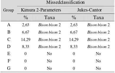
relationships between taxa. For both models, there are only Group A, B, C, and D which have a missedclassification in the original tree. However, the missedclassification rate are really small (Table 7). For those four groups, the taxa of Bison bison 2 is classified wrongly. Based on the taxonomy knowledge, it should be in a cluster of Bison bison. In the phylogenetic tree, it shows an information that

Bison bison 2 is always closer to group of Bos taurus. The distance between Bison bison 2 and Bos taurus is so close and near to 0. For example is in the case of Group B where the distances between Bison bison 2 with Bos taurus 4, 6, and 7 are (0,004), (0,004), (0,009) for both models (Appendix 28). They are relatively small if we compare to other distances. This taxa from its cluster need to be learned more by biologist.

Table 7 Missedclassification Between Taxa in NJ’s Tree for Both Models

Group

Missedclassification Kimura 2-Parameters Jukes-Cantor

% Taxa % Taxa

A 2,63 Bison bison 2 2,63 Bison bison 2 B 6,67 Bison bison 2 6,67 Bison bison 2 C 14,29 Bison bison 2 14,29 Bison bison 2 D 8,33 Bison bison 2 8,33 Bison bison 2

E 0 No 0 No

F 0 No 0 No

G 0 No 0 No

(19)

9

up and went down for a particular group or in unstable condition. In overall replication change from 1.000 to 5.000 Kimura

2-Paramaters, bootstrap confidence value ( is

above 50%. While for Jukes-Cantor, it is below 50%. When the replication change was added up into 5.000-10.000, the value tended to increase for both models. The NJ phylogenetic tree in the repeated times of 5.000-10.000 shows higher consistency than in the repeated times of 1.000-5.000. So, generally it can be concluded that Kimura 2-Parameters performs a better consistency.

Then, NJ’s phylogenetic tree with Kimura 2-Parameters and the Jukes-Cantor model have a good nodes stability. Both of them

have the bootstrap confidence value ( of at

least 0,5 or 50% for the six groups. A comparison of stable nodes percentage for each group has been displayed in Figure 5. There is only one group that has a low proportion of stable nodes and it is Group E. It has a proportion 35,29% (for 1.000 times of bootstrap replication) and 29,41% (for 5.000 and 10.000 times of bootstrap replication). This is caused by the evolutionary distances that are developed in Group E, both for Kimura 2-Parameters or Jukes-Cantor, are small and close to 0, especially in a case ofdistances among Bos indicus (Appendix 24 and Appendix 25). If we compare with another groups (Group A, B, C, D, F, dan G), Group E is involved in a unique case.

Figure 5 A Comparison of Stable Nodes Percentage for Each Group

Both models failed in reconstructing a reliable phylogenetic tree for Group A and G (see Appendix 6 and Appendix 12 for Kimura 2-Parameters; Appendix 13 and Appendix 19 for Jukes-Cantor). Kimura 2-Parameters

shows slightly different topologies

relationships with Jukes-Cantor for Group D and E whereas Kimura 2-Parameters model

could give the constant topologies

relationship, while Jukes-Cantor give the varied tolopogies relationship. In Group B, C,

and F the two models could represent the canstant topologies relationship. In case of topologies relationship, Kimura 2-Parameters models is able to give more constant topologies relationship.

Relating to the condition of being failed in giving a consistence for the topologies, unfortunately, further understanding about this case is needed. Appendix 5 shows the

nucleotide composition’s means and variances

for all built cases. This information shows that compared to other cases, the nucleotide variance for group A and G was relatively small for each nucleotide compositions. The nucleotide variance of Group A for T(U), C, A, G respectively are (1,26), (1,31), (0,82), and (0,47) whereas the composition for Group G are (0,58), (1,32), (1,00), and (0,52). Those are relatively small comparing to group B, C, and F as a groups with constant topologies relationship.

While in group D model Kimura 2-Paramaters showed inconsistency in construct the topologies, especially in describing the

relationship between Bison bison 2, Bos

taurus 1, and Bos taurus 7. When the repeated times are 1.000 and 5.000, Bos taurus 1 and

Bos taurus 7 siblings into a clade and result a

small bootstrap confidence value ( as

many as 30% (for 1.000 replications) and 27% (for 5.000 replication). The clade of Bos taurus 1-Bos taurus 7 then is connected with

Bison bison 2 with a small bootstrap

confidence value ( , 47% (for 1.000

replications) and 45% (for 5.000 replication). This conditions is caused by the nucleotide composition between those three organisms. They have a slight different between Adenines (A) and Guanine (G) where the percentage of Adenines in Bos taurus 1 and Bos taurus 7 is

30% while in Bison bison 2 is 34%.

Otherwise, the percentage of Guanine in Bos taurus 1 and Bos taurus 7 is 15,8% while in

Bison bison 2 is 14,5%. In addition, the percentage of Cytosines (C) and Timine (T) is really different at all. The same thing also happened in Group E where topology relationship among Bos indicus couldn’t be

explained well as we can see from Appendix 10 for Kimura 2-Parameters and Appendix 17 for Jukes-Cantor. In theory, Jukes-Cantor is weaker to cover this condition than Kimura 2-Paramaters because in the reality the event of transversion is more often to happened than transition. Therefore, the substitution rate of

transversion should be different with

(20)

10

As an additional information, the value of BIC also has been computed to compare the

performance of NJ’s tree. BIC has been

widely used to any set of maximum likelihood-based models and developed by Gideon E.S. (Schwarz 1978). At commonly the formula for the BIC is:

where n = the number of observations or equivalently, the sample size; k = the number of free parameters to be estimated; L = the maximized value of the likelihood function for the estimated model. In Appendix 22, Kimura 2-Parameters always has the lower value of BIC than Jukes-Cantor for each group as a built cases. Model with the lower value of BIC is better than those with higher value in the substitution pattern.

CONCLUSION

NJ’s phylogenetic tree with Kimura 2-Parameters and Jukes-Cantor model have a good node stability and is also generally

relationships between taxa. The increasing of bootstrap replication number in common will

increase the consistency of bootstrap

confidence value ( . It means that both

models have a good reliability.

When the number of sequences is large and the extent of sequence divergence is low, the realized tree may have many interior branches with zero length unless a large

number of nucleotides are examined.

Generally it will be difficult to construct the tree by some models. However, phylogenetic tree with Kimura 2-Parameters has a better performance than Jukes-Cantor.

RECOMMENDATION

In order to improve a better knowledge relating to this research topic, some recommendations are given as follow:

1. It would be nice if another distance model

could be applied for the next research.

2. Some built cases can be developed by

combining more various species with more closeness level of various relationship.

REFERENCES

Berry, V and Gascuel O. 1996. Interpretation of bootstrap trees: treshold of clade selection and induced gain. Mol. Biol. Evol. 13: 999-1011.

Efron B, Halloran E, and Holmes S. Bootstrap confidence levels for phylogenetic trees.

1996. Proc. Natl. Acad. Sci. USA

93:7085–7090.

Elfaizi, MA and Aprijani DA. 2004. Bioinformatika: Perkembangan, Disiplin Ilmu, dan Penerapannya di Indonesia. http//www.gnu.org/copyleft/fdl.html. [March10th, 2010]

Hedges, SB. 1992. The number of replications needed for accurate estimation of the

bootstrap p-value in phylogenetics

studies. Mol. Biol. Evol. 9: 366-369. Jukes, TH and Cantor CR. 1969. Evolution of

protein molecules. In Munro HN, editor,

Mammalian Protein Metabolism, pp. 21-132. New York: Academic Press. Kimura, M. 1980. A simple method for

estimating evolutionary rate of base

substitutions through comparative

studies of nucleotide sequences. Journal of Molecular Evolution 16:111-120. Larizza, A et al. 2002. Lineage specificity of

the evolutionary dynamics of the mtDNA D-loop region in rodents.

Journal of Molecular Evolution 54(2): 145-155.

Lesvian, A. 2010. Neighbour Joining and Maximum Likelihood to Cluster Insuline

DNA Sequence [Minithesis]. Department

of Statistics, Faculty of Mathematics and Netural Sciences, IPB. Bogor.

Li Yan. 2001. How to build a phylogenetic

tree. http://hiv-web.lanl.gov/.

[March10th, 2011].

Nei, M and Kumar S. 2000. Molecular

evolution and phylogenetics. New York: Oxford University Press.

Otu, HH and Sayood K. 2003. A new

sequence distance measure for

phylogenetic tree construction. Journal of Bioinformatics 19: 2122-2130. Putri, D.R. 2010. Molecular phylogenetic tree

using three different methods based on

p-distance model [Minithesis].

Department of Statistics, Faculty of Mathematics and Natural Sciences, IPB. Bogor.

Saitou, N and Nei M.1987.The Neighbour Joining method: a new method for reconstructing phylogenetic trees. Mol. Biol. Evol. 4: 406-425.

Schwarz, Gideon E. 1978. Estimating the

dimension of a model. Annals of

Statistics 6(2): 461–464.

Soltis, P.S and Soltis D.E. 2003.Applying the bootstrap in phylogeny reconstruction.

(21)

Appendix 1 Spesification of D-loop mtDNA Sequences for All Organisms

>Bison_bison(1)

TCCAATAACTCAACACAAACTTTGTACTCTAACCAAATATTGCAAACACCACTAGCTA ACGTCACTCACCCCAAAATGCATTACCCAAACGGGGGAATATACATAACATTAATGT AATAAAAACATATTATGTATATAGTACATTAAATTATATGCCCCATGCATATAAGCAA GTACTTATCCTCTATTGACAGTACATAGTACATAAAGTTATTAATTGTACATAGCACA TTATGTCAAATCTACCCTTGGCAACATGCATATCCCTTCCATTAGATCACGAGCTTAAT TACCATGCCGCGTGAAACCAGCAACCCGCTAGGCAGAGGATCCCTCTTCTCGCTCCGG GCCCATGAACCGTGGGGGTCGCTATTTAATGAACTTTATCAGACATCTGGTTCTTTCTT C

>Bison_bison(2)

CACAGAATTTGCACCCTAACCAAATATTACAAACACCACTAGCTAACATAACACGCCC ATACACAGACCACAGAATGAATTACCTACGCAAGGGGTAATGTACATAACATTAATG TAATAAAGACATAATATGTATATAGTACATTAAATTATATGCCCCATGCATATAAGCA AGTACATGACCTCTATAGCAGTACATAATACATATAATTATTGACTGTACATAGTACA TTATGTCAAATTCATTCTTGATAGTATATCTATTATATATTCCTTACCATTAGATCACG AGCTTAATTACCATGCCGCGTGAAACCAGCAACCCGCTAGGCAGGGATCCCTCTTCTC GCTCCGGGCCCATAAACCGTGGGGGTCGCTATCCAATGAATTTTACCAGGCATCTGGT TCTTTCTTC

>Bison_bison(3)

TCCAATAACTCAACACAAACTTTGTACTCTAACCAAATACTGCAAACACCACTAGCTA ACGTCACTCACCCCCAAAATGCATTACCCAAACGGGGGGAAATATACATAACATTAA TGTAATAAAAACATATTATGTATATAGTACATTAAATTATATGCCCCATGCATATAAG CAAGTACTTATCCTCTATTGACAGTACATAGTACATAAAGTTATTAATTGTACATAGC ACATTATGTCAAATCTACCCTTGGCAACATGCATACCCCTTCCATTAGATCACGAGCT TAATTACCATGCCGCGTGAAACCAGCAACCCGCTAGGCAGAGGATCCCTCTTCTCGCT CCGGGCCCATGAACCGTGGGGGTCGCTATTTAATGAACTTTATCAGACATCTGGTTCT TTCTTC

>Bos_taurus(1)

CCCCATGCATATAAGCAAGTACATGACCTCTATAGCAGTACATAATACATATAATTAT TGACTGTACATAGTACATTATGTCAAATTCATTCTTGATAGTATATCTATTATATATTC CTTACCATTAGATCACGAGCTTAATTACCATGCCGCGTGAAACCAGCAACCCGCTAGG CAGGGATCCCTCTTCTCGCTCCGGGCCCATAAACCGTGGGGGTCGCTATCCAATGAAT TTTACCA

>Bos_taurus(2)

CCCCATGCATATAAGCAAGTACATGACTTCTATAGCAGTACATAATACATATAATTAT TGACTGTACATAGTACATTATGTCAAATTCATCCTTGATAGTATATCTATTATATATTC CTTACCGTTAGATCACGAGCTTAATTACCATGCCGCGTGAAACCAGCAACCCGCTAGG CAGGGATCCCTCTTCTCGCTCCGGGCCCATAAATCGTGGGGGTCGCTATTCAATGAAC TTTACCA

>Bos_taurus(3)

(22)

CAGGGATCCCTCTTCTCGCTCCGGGCCCATAAACCGTGGGGGTCGCTATCCAATGAAT TTTACCA

>Bos_taurus(4)

CCCCATGCATATAAGCAAGTACATGACCTCTATAGCAGTACATAATACATATAATTAT TGACTGTACATAGTACATTATGTCAAATTCATTCTTGATAGTATATCTATTATATATTC CTTACCATTAGATCACGAGCTTAATTACCATGCCGCGTGAAACCAGCAACCCGCTAGG CAGGGATCCCTCTTCTCGCTCCGGGCCCATAAACCGTGGGGGTCGCTATCCAATGAAT TTTATCA

>Bos_taurus(5)

CCCCATGCATATAAGCAAGTACATGACCTCTATAGCAGTACATAATACATATAATTAT TGACTGTACATAGTACATTATGTCAAATTCATTCTTGATAGTATATCTATTATATATTC CTTACCATTAGATCACGAGCTTAATTACCATGCCGCGTGAAACCAGCAACCCGCTAGG CAGGGATCCCTCTTCTCGCTCCGGGCCCATAAACCGTGGGGGTCGCTATCCAATGAAT TTTATCA

>Bos_taurus(6)

CCCCATGCATATAAGCAAGTACATGACCTCTATAGCAGTACATAATACATATAATTAT TGATTGTACATAGTACATTATGTCAAATTCATTCTTGATAGTATATCTATTATATATTC CTTACCATTAGATCACGAGCTTAATTACCATGCCGCGTGAAACCAGCAACCCGCTAGG CAGGGATCCCTCTTCTCGCTCCGGGCCCATAAACCGTGGGGGTCGCTATCCAATGAAT TTTACCA

>Bos_taurus(7)

CCCCATGCATATAAGCAAGCACATGACCTCTATAGCAGTACATAATACATATAATTAT TGACTGTACATAGTACATTATGTCAAATTCACTCTTGATAGTATATCTATTATATATTC CTTACCATTAGATCACGAGCTTAATTACCATGCCGCGTGAAACCAGCAACCCGCTAGG CAGGGATCCCTCTTCTCGCTCCGGGCCCATAAACCGTGGGGGTCGCTATCCAATGAAT TTTACCA

>Bos_taurus(8)

CCCCATGCATATAAGCAAGTACATGACCTCTATAGCAGTACATAATACATACAATTAT TGACTGTACATAGTACATTATGTCAAATTCATCCTTGATAGTATATCTATTATATATTC CTTACCATTAGATCACGAGCTTAATTACCATGCCGCGTGAAACCAGCAACCCGCTAGG CAGGGATCCCTCTTCTCGCTCCGGGCCCATAAACCGTGGGGGTCGCTATCTAATGAAC TTTACCA

>Bos_indicus(1)

(23)

>Bos_indicus(2)

GCAAGAGGTAATGTACATAACATTAATGTAATAAAGACATGATATGTATATAGTACA TTAAATTATATACCCCATGCATATAAGCAAGTACATGATCTCTATAATAGTACATAAT ACATACAATTATTAATTGTACATAGTACATTATATCAAATCCATCCTCAACAACATAT CTACTATATACCCCTTCCACTAGATCACGAGCTTAATTACCATGCCGCGTGAAACCAG CAACCCGCTAAGCAAAGGATCCCTCTTCTCGCTCCGGGCCCATAGACCGTGGGGGTCG CTATTTAATGAATTTTACCAGGCATCTGGTTCTTTCTTCAGGGCCATCTCATCTAAAGT GGTCCATTCTTTCCTCTTAAATAAAACATCTCGATGGACTAATGACTAATCAGCCCAT GCTCACACATAACTGTGCTGTCATACATTTGGTATTTTTTTATTTTGGG

>Bos_indicus(3)

GCAAGAGGTAATGTACATAACATTAATGTAATAAAGACATGATATGTATATAGTACA TTAAATTATATACCCCAGGCATATAAGCAAGTACATGATCTCTATAATAGTACATAAT ACATACAATTATTAATTGTACATAGTACATTATATCAAATCCATCCTCAACAACATAT CTACTATATACCCCTTCCACTAGATCACGAGCTTAATTACCATGCCGCGTGAAACCAG CAACCCGCTAAGCAAAGGATCCCTCTTCTCGCTCCGGGCCCATAGACCGTGGGGGTCG CTATTTAATGAATTTTACCAGGCATCTGGTTCTTTCTTCAGGGCCATCTCATCTAAAGT GGTCCATTCTTTCCTCTTAAATAAAACATCTCGATGGACTAATGACTAATCACCCCAT GCTCACACATAACTGTGCTGTCATACATTTGGTATTTTTTTATTTTGGG

>Bos_indicus(4)

GCAAGAGGTAATGTACATAACATTAATGTAATAAAGACATGATATGTATATAGTACA TTAAATTATATACCCCATGCATATAAGCAAGTACATGATCTCTATAATAGTACATAAT ACATACAATTATTAATTGTACATAGTACATTATATCAAATCCATCCTCAACAACATAT CTACTATATACCCCTTCCACTAGATCACGAGCTTAATTACCATGCCGCGTGAAACCAG CAACCCGCTAAGCAGAGGATCCCTCTTCTCGCTCCGGGCCCATAGACCGTGGGGGTCG CTATTTAATGAATTTTACCAGGCATCTGGTTCTTTCTTCAGGGCCATCTCATCTAAAGT GGTCCATTCTTTCCTCTTAAATAAGACATCTCGATGGACTAATGACTAATCAGCCCAT GCTCACACATAACTGTGCTGTCATACATTTGGTATTTTTTTATTTTGGG

>Bos_indicus(5)

>Bos_indicus(6)

(24)

>Bos_indicus(7)

GCAAGAGGTAATGTACATAACATTAATGTAATAAAGACATGATATGTATATAGTACA TTAAATTATATACCCCATGCATATAAGCAAGTACATGATCTCTATAATAGTACATAAT ACATACAATTATTAATTGTACATAGTACATTATATCAAATCCATCCTCAACAACATAT CTACTATATACCCCTTCCACTAGATCACGAGCTTAATTACCATGCCGCGTGAAACCAG CAACCCGCTAAGCAAAGGATCCCTCTTCTCGCTCCGGGCCCATAGACCGTGGGGGTCG CTATTTAATGAATTTTACCAGGCATCTGGTTCTTTCTTCAGGGCCATCTCATCTAAAGT GGTCCATTCTTTCCTCTTAAATAAAACATCTCGATGGACTAATGACTAATCAGCCCAT GCTCACACATAACTGTGCTGTCATACATTTGGTATTTTTTTATTTTGGG

>Bos_indicus(8)

>Bos_indicus(9)

GCAAGAGGTAATGTACATAACATTAATGTAATAAAGACATGATATGTATATAGTACA TTAAATTATATACCCCATGCATATAAGCAAGTACATGATTTCTATAATAGTACATAAT ACATACAATTATTAATTGTACATAGTACATTATATCAAATCCATCCTCAACAACATAT CTACTATATACCCCTTCCACTAGATCACGAGCTTAATTACCATGCCGCGTGAAACCAG CAACCCGCTAAGCAGAGGATCCCTCTTCTCGCTCCGGGCCCATAGACCGTGGGGGTCG CTATTTAATGAATTTTACCAGGCATCTGGTTCTTTCTTCAGGGCCATCTCATCTAAAGT GGTCCATTCTTTCCTCTTAAATAAGACATCTCGATGGACTAATGACTAATCAGCCCAT GCTCACACATAACTGTGCTGTCATACATTTGGTATTTTTTTATTTTGGG

>Bos_indicus(10)

GCAAGAGGTAATGTACATAACATTAATGTAATAAAGACATGATATGTATATAGTACA TTAAATTATATACCCCATGCATATAAGCAAGTACATGATCTCTATAATAGTACATAAT ACATACAATTATTAATTGTACATAGTACATTATATCAAATCCATTCTCAACAACATAT CTACTATATACCCCTTCCACTAGATCACGAGCTTAATTACCATGCCGCGTGAAACCAG CAACCCGCTAAGCAGAGGATCCCTCTTCTCGCTCCGGGCCCATAGACCGTGGGGGTCG CTATTTAATGAATTTTACCAGGCATCTGGTTCTTTCTTCAGGGCCATCTCATCTAAAGT GGTCCATTCTTTCCTCTTAAATAAGACATCTCGATGGACTAATGACTAATCAGCCCAT GCTCACACATAACTGTGCTGTCATACATTTGGTATTTTTTTATTTTGGG

>Bos_indicus(11)

(25)

>Bos_indicus(12)

GCAAGAGGTAATGTACATAACATTAATGTAATAAAGACATGATATGTATATAGTACA TTAAATTATATACCCCATGCATATAAGCAAGTACATGATCTCTATAATAGTACATAAT ACATACAATTATTAATTGTACATAGTACATTATATCAAATCCATCCTCAACAACATAT CTACTATATACCCCTTCCACTAGATCACGAGCTTAATTACCATGCCGCGTGAAACCAG CAACCCGCTAAGCAGAGGATCCCTCTTCTCGCTCCGGGCCCATAGACCGTGGGGGTCG CTATTTATTGAATTTTACCAGGCATCTGGTTCTTTCTTCAGGGCCATCTCATCTAAAGT GGTCCATTCTTTCCTCTTAAATAAGACATCTCGATGGACTAATGACTAATCAGCCCAT GCTCACACATAACTGTGCTGTCATACATTTGGTATTTTTTTATTTTGGG

>Bos_indicus(13)

>Bos_indicus(14)

>Bos_indicus(15)

GCAAGAGGTAATGTACATAACATTAATGTAATAAAGACATAATATGTATATAGTACA TTAAATTATATACCCCATGCATATAAGCAAGTACATGATCTCTATAATAGTACATAAT ACATACAATTATTAATTGTACATAGTACATTATATCAAATCCATCCTCAACAACATAT CTACTATATACCCCTTCCACTAGATCACGAGCTTAATTACCATGCCGCGTGAAACCAG CAACCCGCTAAGCAGAGGATCCCTCTTCTCGCTCCGGGCCCATAGACCGTGGGGGTCG CTATTTAATGAATTTTACCAGGCATCTGGTTCTTTCTTCAGGGCCATCTCATCTAAAGT GGTCCATTCTTTCCTCTTAAATAAGACATCTCGATGGACTAATGACTAATCAGCCCAT GCTCACACATAACTGTGCTGTCATACATTTGGTATTTTTTTATTTTGGG

>Bos_indicus(16)

(26)

>Bos_grunniens_mutus(1)

AACGCTATTAATATAGTTCCATAAATGTAAAGAGCCTCACCAGTATTAAATTTACTAA AAATTCCAATAACTCAACACAAACTTTGTACTCTAACCAAATATTACAAACTCCACTA ACTAACAACACACATCCCTAAAAATACATTGTCCAAACGGGGGATACGTACATAATA TTAATGTAATAAAAACATACTATGTATATAGTACATTAAATTATTTACCCCATGCATA TAAGCAAGTACATAATCTCTATTAATAGTACATAGTACATGAAGTTATTAATCGTACA TAGCACATTATGTCAAACTCACTCCTGACAACATGCATACCCCTTCCACTAGATCACG AGCTTAATTACCATGCCGCGTGAAACCAGCAACCCGCTAGGCAAAGGACTCCTCTTCT CGCTCCGGGCCCATGAACTGTGGGGGTCGCTATTTAATGAACTTTATCAGACATCTGG TTCTTTCTTCAGGGCCATCTCACCTAAAACCGTCCATTCTTTCCTCTTAAATAAGACAT CTCGATGGACTAATGACTAATCAGCCCATGCTCACACATAACTGTGCTGTCATACATT TGGTATTTTTTTATTTTGGGGGATGCTTGGACTCAGCTATGGCCGTCAAAGGCCCCGA CCCGGAGCATCTATTGTAGCTGGACTTAACTGCATCTTGAGCACCAGCATAATGGTAA GCATGCACATATAGTCAATGGTTACAGGACATAAATTATATTATATATCCCCCCCTCC ATAAAAATTCCCCCTTAAATATTTACCACTACTTTTAACAGATTTTTCCCTAGTTACTT ATTTAAAATTTCCACACTTTCAATACTCAAATTAGCACTCCATATAAAGTCAATATAT AAACGCAGGCCCCCCCCCCCCC

AACGCTATTAATATAGTTCCATAAATGTAAAGAGCCTCACCAGTATTAAATTTACTAA AAATTCCAATAACTCAACACAAACTTTGTACTCTAACCAAATATTACAAACACCACTA GCTAACAACACACATCCCCAAAAATGCATTGTCCAAACGGGGGAATACGTACATAAT ATTAATGTAATAAAGACATATTATGTATATAGTACATTAAATTATATGCCCCATGCAT ATAAGCAAGTACATAATTCCTATTGGTAGTACATAGTACATGAAATTATTAATCGTAC ATAACATATTATGTCAAACCTACTCCTAACAACATGTATACCCCCTCCACTAGATCAC GAGCTTAACTACCATGCCGCGTGAAACCAGCAACCCGCTAGGCGGAGGACTCCTCTTC TCGCTCCGGGCCCATGAACTGTGGGGGTCGCTATTTAATGAACTTTATCAGACATCTG GTTCTTTCTTCAGGGCCATCTCACCTAAAACCGTCCACTCTTTCCTCTTAAATAAGACA TCTCGATGGACTAATGGCTAATCAGCCCATGCTCACACATAACTGTGCTGTCATACAT TTGGTATTTTTTTATTTTGGGGGATGCTTGGACTCAGCTATGGCCGTCAAAGGCCCCGA CCCGGAGCATCTATTGTAGCTGGACTTAACTGCATCTTGAGCACCAGCATAATGATAG GCATGCACATATAGTCAATGGTCACAGGACATAGATTATATTATATATCCCCCCCTCC ATAAAAATTCCCCCTTAAATATTTACCACTACTTTTAACAGATTTTTCCCTAGTTGCTT ATTTAAAATTTCCACACTTTCAATACTCAAATTAGCACTCCATATAAAGTCAATATAT AAACGCAGGCCCCCCCCCCCCC

(27)

ATAAAAATTCCCCCTTAAATATTTACCACTACTTTTAACAGATTTTTCCCTAGTTACTT ATTTAAAATTTCCACACTTTCAATACTCAAATTAGCACTCCATATAAAGTCAATATAT AAACGCAGGCCCCCCCCCCCC

AACGCTATTAATATAGTTCCATAAATGTAAAGAGCCTCACCAGTATTAAATTTACTAA AAATTCCAATAACTCAACACAAACTTTGTACTCTAACCAAATATTACAAACACCACTA GCTAACAACACACATCCCTAAAAATACATTGTCCAAACGGGGGATACGTACATAATA TTAATGTAATAAAAACATACTATGTATATAGTACATTAAATTATATGCCCCATGCATA TAAGCAAGTACATAATCCCTATTAATAGTACATAGTACATGAAGTTATTAATCGTACA TAGCACATTATGTCAAACTCGCTCCTGACAACATGCATACCCCTTCCACTAGATCACG AGCTTAACTACCATGCCGCGTGAAACCAGCAACCCGCTAGGCAAAGGACTCCTCTTCT CGCTCCGGGCCCATGAACTGTGGGGGTCGCTATTTAATGAACTTTATCAGACATCTGG TTCTTTCTTCAGGGCCATCTCACCTAAAACCGTCCATTCTTTCCTCTTAAATAAGACAT CTCGATGGACTAATGACTAATCAGCCCATGCTCACACATAACTGTGCTGTCATACATT TGGTATTTTTTTATTTTGGGGGATGCTTGGACTCAGCTATGGCCGTCAAAGGCCCCGA CCCGGAGCATCTATTGTAGCTGG