1
MODELING SPATIAL DYNAMIC OF CORAL REEF ON THE
SMALL ISLAND, SPERMONDE ARCHIPELAGO
Case Study: Barrang Lompo Island, Makassar District, Indonesia
AGUS
GRADUATE SCHOOL
BOGOR AGRICULTURAL UNIVERSITY BOGOR
STATEMENT
I, Agus, hereby declare that this thesis entitled
Modeling Spatial Dynamic of Coral Reef on the Small Island, Spermonde Archipelago (Case Study: Barrang Lompo Island, Makassar
District, Indonesia)
Is a result of my work under the supervision advisory board and that it has not been published before. The content of this thesis has been examined by the advisory board and external examiner.
Bogor, April 2014
Agus
3
RINGKASAN
AGUS. Permodelan Dinamika Spasial Terumbu Karang di Pulau Pulau Kecil, Kepulauan Spermonde (Studi Kasus: Pulau Barrang Lompo, Kota Makassar, Indonesia). Dibawah bimbingan oleh VINCENTIUS P SIREGAR dan IBNU SOFIAN.
Terumbu karang di Coral Triangle Asia sampai sekarang terancam oleh aktivitas manusia dan ancaman alam. Kerusakan terumbu karang juga terjadi di kepulauan Spermonde khususnya pulau Barrang Lompo (COREMAP II 2010). Pulau Barrang Lompo memberikan kontribusi tinggi terhadap masyarakat, sebagian besar mata pencahariannya bergantung pada perairan dangkalnya. Oleh karena itu, pemetaan dinamika spasial dan prediksi tren masa depan terumbu karang diperlukan untuk membuat perencanaan tata ruang untuk daerah pesisir dengan menggunakan data penginderaan jauh dan model M-CA. Adapun tujuan dari penelitian ini adalah menganalisis dinamika spasial terumbu karang dengan menggunakan data penginderaan jauh dan prediksi tren masa depan perubahan terumbu karang.
Penelitian ini dilakukan dari bulan November 2012 sampai Desember 2013 di perairan Pulau Barrang Lompo. Ada beberapa data yang digunakan di penelitian ini. Landsat TM / ETM + tahun 1993 , 1997 , 2002 , 2007, dan 2012 telah di proses menggunakan klasifikasi untuk membuat sebuah peta terumbu karang. Peta probabilitas diperoleh dari perkalian peta salinitas, SST, DO, pH, TSS, kecerahan, batimetri, dan peta constraint yang merupakan daratan dan perairan laut dalam di Pulau Barrang lompo yang diasumsikan tidak akan berubah menjadi terumbu karang untuk jangka waktu 10 tahun.
Penelitian ini telah dilakukan dalam beberapa langkah; a) survei lapangan, b) pengolahan citra, c) analisis rantai Markov, d) analisis MCE, e) analisis CA, f) validasi dan, g) prediksi perubahan terumbu karang. Data dari lapangan telah digunakan untuk pengolahan citra. Hal ini diterapkan pada jenis habitat yang diperlukan dari seluruh wilayah studi dengan menggunakan GPS. Pengolahan citra digunakan untuk klasifikasi peta terumbu karang pada berbeda waktu. Hasil klasifikasi digunakan sebagai masukan analisis rantai Markov untuk mendapatkan
transition area matrix. Analisis MCE digunakan membuat peta probabilitas dengan menggunakan beberapa parameter. Hasil pengolahan citra, hasil analisis rantai Markov dan hasil MCE digunakan sebagai masukan untuk melakukan model CA. Hasil simulasi CA divalidasi dengan peta sebenarnya yang diperoleh dari citra Landsat untuk mengevaluasi hasil prediksi. Jika hasil validasi >75%, kemudian memprediksi tren masa depan terumbu karang 10 tahun ke depan.
2007 sampai 2012, sementara karang mati, pecahan karang, dan pasir meningkat dari tahun 1993 sampai 2012. Berdasarkan pengamatan lapangan, kerusakan habitat terumbu karang di Pulau Barrang Lompo sebagian besar disebabkan oleh aktivitas manusia, hal ini terbukti dari banyaknya fragmen batuan (pecahan karang), dan kegiatan penangkapan ikan menggunakan bahan peledak/bom dan bahan kimia oleh nelayan (Coremap II 2010). Menurut Yusuf dan Jompa (2012), fenomena pemutihan karang juga terjadi pada akhir tahun 2009 sampai pertengahan tahun 2010 yang disebabkan dari fenomena La Nina yang meningkatkan SST oleh gerakan warmpool ke arah barat dari Pasifik Tengah ke Laut Indonesia, karena penguatan angin pasat yang secara signifikan menurunkan kualitas terumbu karang di kepulauan Spermonde.
Hasil simulasi perubahan terumbu karang yang menggunakan nilai 5 sebagai total iterasi, dan jenis filtering 5x5 digunakan untuk memprediksi tahun 2002, 2007 dan 2012. Sementara untuk memprediksi 2022 digunakan nilai 10 sebagai iterasi. Sebelum memprediksi tahun 2022, hasil simulasi perubahan terumbu karang tahun 2002, 2007, dan 2012 dibandingkan antara hasil klasifikasi terumbu karang yang diperoleh dari citra. Penelitian ini menggunakan KIA dan secara distribusi spasial digunakan Post-Classification untuk melihat akurasi model. Hasil perhitungan overall kappa diperoleh adalah 2002 (89,41 %), 2007 (88,86%), 2012 (87,71%). Meskipun hasil model M-CA di setiap tahun terdapat over-estimasi, namun nilai validasi cukup baik untuk memprediksi tren masa depan terumbu karang untuk tahun 2022 karena prestasi yang lebih tinggi dari nilai standar 75 % (Montserud et al. 1992 in Wassahua 2010). Berdasarkan hasil simulasi tren perubahan terumbu karang dari tahun 2012 sampai 2022, total luasan terumbu karang di prediksi menurun dari 78,86 ha menjadi 63,55 ha. Dalam hal ini, terumbu karang memiliki tingkat perubahan yang lebih tinggi dan jika hal ini selalu terjadi maka kawasan terumbu karang akan hilang. Di sisi lain, karang mati dan pecahan karang di prediksi meningkat masing-masing 5,86 ha menjadi 15,83 ha dan 7,48 ha menjadi 13,62 ha.
Dari hasil dan pembahasan, kesimpulan dapat digambarkan sebagai berikut. Kondisi karang hidup menurun dari tahun 1993 sampai 2012. Penurunan terbesar terjadi pada tahun 2002 sampai 2007 tutupan sebesar 4.51 ha dan penurunan terbesar kedua terjadi pada tahun tahun 2007 sampai 2012 sebesar 4.15 ha. Relatif luas karang hidup cenderung menjadi karang mati dan pecahan karang. Hasil model M-CA menunjukkan kondisi karang hidup dari tahun 2012 sampai tahun 2022 diprediksi mengalami penurunan sekitar 15,31 ha (19,41%), dan karang mati dan pecahan karang di prediksi bertambah dari 5.86 ha menjadi 15.83 ha dan 7.48 ha menjadi 13.62 ha, Selain itu, rekomendasi dari penelitian ini parameter SST digunakan sebagai skenario, hasil dari model spasial M-CA dapat digunakan untuk prediksi masa depan perubahan terumbu karang. Namun model ini tidak belum menggunakan aktifitas manusia sebagai masukan. Jadi penelitian selanjutnya untuk prediksi masa depan terumbu karang sebaiknya menggunakan model yang mempertimbangkan aktivitas manusia sebagai masukan.
SUMMARY
AGUS. Modeling Spatial Dynamic of Coral Reef on the Small Island, Spermonde Archipelago (Case Study: Barrang Lompo Island, Makassar District Indonesia). Under the supervisor of VINCENTIUS P SIREGAR and co-supervisor of IBNU SOFIAN.
The coral reef in the Coral Triangle Asia has been directly threatened by human activities and natural threats. The coral reef destructions have also happened in Spermonde Archipelago especially Barrang Lompo Island (COREMAP II 2010). Barrang Lompo Island contributes highly to the society, the most livelihoods of which depends on its shallow water. Therefore, spatial dynamic mapping and spatial prediction model for future trend of coral reef are needed to create good spatial planning for coastal area using remote sensing data and M-CA Model. The objective of this research was to analyze dynamics of coral reef by using remote sensing data and also to predict the future trend of coral reef change.
The research was conducted from November 2012 to December 2013 at the shallow water of Barrang Lompo Island. There are several data used in this study. Landsat TM / ETM+ of 1993, 1997, 2002, 2007, and 2012 were processed using image classification for coral reef map. Probability maps were derived from multiplication maps of salinity, sea surface temperature (SST), Dissolve Oxygen (DO), pH, total suspended sediment (TSS), water clearness, bathymetry, and the constraint map used were land area and deep water in Barrang lompo with the assumption that the area will not change into coral reef for 10 years.
This research has been conducted in several steps: a) ground truth, b) image processing, c) Markov chain analysis, d) Multi criteria evaluation (MCE) analysis, e) Cellular Automata (CA) analysis, f) validation and, g) coral reef change prediction. The main measurement data was derived from ground truth. Ground truth data from the field were used for image processing. They were applied on the required habitat types of the whole study area by using Global Position System (GPS). Image processing was used to classify coral reef at different times. The classified images were used as input for Markov chain analysis in order to get transition area matrix. MCE analysis was used to create a probabilities map using several parameters. The results of image processing, Markov chain analysis and MCE were used as inputs to perform the CA model. The final result of this model was the coral reef change prediction. The result of simulation from CA process was validated using the actual coral reef map obtained from Landsat image to evaluate the prediction result. If the result validation standard agreement is >75%, then it can be used to predict the future trend coral reef for the next 10 years.
4.15 ha and 1.46 ha from 2007 to 2012, respectively. While dead coral, rubble, and sand has been from 1993 to 2012. Based on observations in the field, the coral reef habitat destruction in Barrang Lompo Island was largely caused by human activities. It was proven by many fragments of rock (rubble), and the activities by explosives fishing such as bombs and chemicals in shallow waters Barrang Lompo (COREMAP II 2010). According to Yusuf and Jompa (2012), the phenomenon of coral bleaching that occurred at the end of 2009 until middle of 2010 was caused by La Nina phenomena increasing the SST by the westward warmpool movement from the Central Pacific to the Indonesian Seas, due to the strengthening of trade winds that significantly decreased the quality of coral reefs in the Spermonde archipelago.
The simulation result of coral reef change used the number 5 times as the total iterations, and filtering type 5x5 cell contiguity filtering was used to predict in 2002, 2007 and 2012, while to predict 2022 the number 10 iterations was used. Before simulation model to predict in 2022, the simulation result of coral reef change of 2002, 2007, and 2012 then compared with classification result of coral reef obtained from Landsat images. This study used Kappa Index Agreement (KIA) and spatial distribution was indicated by Post-Classification to see the accuracy of model. Calculation results obtained were 2002 (89.41%), 2007 (88.86%), 2012 (87.71%) overall kappa. Although the results of the model M-CA every year was over-estimated, the value of validation was good enough to predict the future trend of coral reef of 2022 because the achievement was higher than the standard value of 75% (Montserud et al. 1992 in Wassahua 2010). Based on the simulation model trend of coral reef change from 2012 to 2022, the total area of coral reef was predicted to decrease from 78.86 ha to 63.55 ha. In this case, coral reef had a higher change rate and if it always occurs the coral reef area will disappear or be broken in Barrang Lompo Island. On the other hand, dead coral and rubble were predicted to increase from 5.86 ha to 15.83 ha and 7.48 ha to 13.62 ha, respectively.
From the fore going discussion, the conclusion can be described as follows. The live coral condition decreased from 1993 to 2012. The greatest decreases occurred from 2002 to 2007 covering about 4.51 ha and second greatest decreases was from 2007 to 2012 about 4.15 ha. Relatively live coral areas tend to become dead coral and rubber. The result model M-CA showed the condition of live coral area from 2012 to 2022 was predicted to decrease about 15.31 ha (19.41%), and dead coral and rubble predicted to increase from 5.86 ha to 15.83 ha and 7.48 ha to 13.62 ha, respectively. Furthermore, the recommendation from this research is that SST parameters was used as a scenario, the result of this spatial model M-CA can be used to predict the future trend of coral reef change. However, this model has not used human activity parameter as input. Hence, future research on predicting the future trend of coral reef should use a model that considers the human activities as input.
Copyright © 2014, Bogor Agricultural University
Copyright are protected by law
It is prohibited to cite all or part of this thesis without referring to and mentioning the source; Citation only permitted for the sake of education, research, scientific writing, critical writing or reviewing scientific problems.
Citation does not inflict the name and honor of Bogor Agricultural University.
A Thesis submitted for the Degree of Master of Science in Information Technology for Natural Resources
Management Program Study
MODELING SPATIAL DYNAMIC OF CORAL REEF ON THE
SMALL ISLAND, SPERMONDE ARCHIPELAGO
Case Study: Barrang Lompo Island, Makassar District, Indonesia
GRADUATE SCHOOL
BOGOR AGRICULTURAL UNIVERSITY BOGOR
Research Title : Modeling Spatial Dynamic of Coral Reef on The Small Island, Spermonde Archipelago (Case Study : Barrang Lompo Island, Makassar District, Indonesia)
Name : Agus
Student ID : G051110011
Approved by,
Advisory Board
Dr Ir Vincentius P. Siregar, DEA Supervisor
Dr Ibnu Sofian, MEng Co-Supervisor
Endorsed by,
Program Coordinator of MSc in IT for Natural Resources
Management
Dr Ir Hartrisari Hardjomidjojo, DEA
Dean of Graduate School
Dr Ir Dahrul Syah, MScAgr
Date of examination:
January 28, 2014
ACKNOWLEDGEMENT
Alhamdulillahi Robbil Alamiin, Praise be to Allah SWT The Greatest, Lord of the World, The All-Wise. Grateful for all of Your grace, I could finish my thesis successfully. The success of this study would not have been possible without various contribution and support from many people, and I will not be able to mention them one by one. Of course, I would like to express my highly appreciation to the following:
1. My family for giving the unwavering faith and supporting me to finish my master degree
2. Dr Ir Vincentius P. Siregar, DEA as my supervisor and Dr Ibnu Sofian, MEng as the co-supervisor for their ideas, comments and constructive criticism during my research.
3. Dr Ir Suria Darma Tarigan, MSc and Dr Bib Paruhum Silalahi as the external examiner for his positive inputs and ideas.
4. Dr Ir Hartrisari Hardjomidjojo, DEA, as the program coordinator and all my teachers, my lectures for giving knowledge and experience.
5. Dr Nurjannah Nurdin, ST, MSi for helping provide data and suggestions during my research.
6. All my friends at MIT IPB class of 2011 for helping, supporting, and togetherness in finishing our assignment and study during our time in pursuing our master degree.
7. All my friends at Graduate Bachelor in Marine Science class 2006 for supporting and helping.
8. MIT secretariat and its staff for helping me to arrange the administration, technical procedures and facilities.
9. Bapak Purwanto as Head Observation Division and Marine Meteorological information Makassar for providing information oceanography data in my research.
Hopefully, this thesis could give positive contribution to anyone who reads it.
Bogor, April 2014
LIST OF CONTENTS
LIST OF TABLES vii
LIST OF FIGURES vii
LIST OF APPENDICES viii
1. INTRODUCTION
Background 1
Objectives 2
Problem Formulation 3
2. LITERATURE REVIEW
Coral Reef 3
Remote Sensing Technique for Shallow Water 4
Total Suspended Sediment (TSS) 6
Sea Surface Temperature (SST) 6
Markov Chain 7
Cellular Automata (CA) 8
3. METHODOLOGY
Time and Location of the Research 10
Material 11
Method 11
4. RESULT AND DISCUSSION
Image Processing 22
Geometric Correction 22
Image Processing 22
Accuracy Assessment 25
Coral Reef Change Predictions 25
Markov Chain Analyses 25
Multi Criteria Evaluation (MCE) 28
Cellular Automata Model 30
5. CONCLUSION AND RECOMMENDATION
Conclusion 33
Recommendation 33
REFERENCES 33
APPENDICES 37
LIST OF TABLES
Table 1 Remote sensing technique for coral reef mapping 5
Table 2 Types of data and sources 11
Table 3 The criteria of coral cover 12
Table 4 Confusion matrix 14
Table 5 Transition area matrix of coral reef area 17 Table 6 Transition probability matrix of coral reef area 18 Table 7 Criteria and categorization of factor coral reef change 19 Table 8 Area calculation for coral reef map 1993 to 2012 22 Table 9 Changes in coral reef areas between in 1993 to 2012 23 Table 10 Confusion matrix for coral reef classification in 2012 25 Table 11 Transition probability to predict coral reef condition in 2002 25 Table 12 Transition area to predict coral reef condition in 2002 26 Table 13 Transition probability to predict coral reef condition in 2007 26 Table 14 Transition area to predict coral reef condition in 2007 26 Table 15 Transition probability to predict coral reef condition in 2012 27 Table 16 Transition area to predict coral reef condition in 2012 27 Table 17 Transition probability to predict coral reef condition in 2022 27 Table 18 Transition area to predict coral reef condition in 2022 28 Table 19 Area Statistics for coral reef change from classification in 2012
and simulation of the future trend coral reef change 2022 32
LIST OF FIGURES
Figure 1 Reflectance spectral of coral reef benthic organism (coral and algae) and observation bands for Landsat TM. Spectral feature
of coral is indicate d by an arrow 5
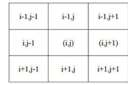
Figure 2 The neighbored from cell (i,j) is formed from Cells (i,j) itself
and eight (8) surrounding cells 9
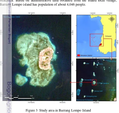
Figure 3 Study area in Barrang Lompo Island 10
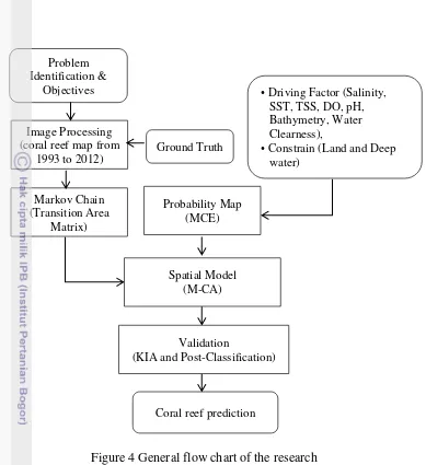
Figure 4 General flow chart of the research 12
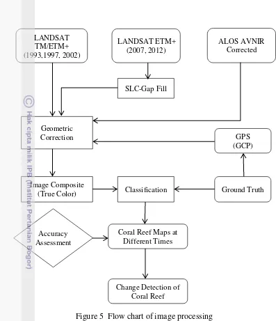
Figure 5 Flow chart of image processing 14
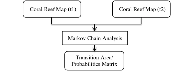
Figure 6 Flow diagram of Markov chain model 17
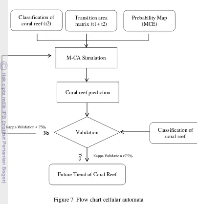
Figure 7 Flow chart cellular automata 21
Figure 8 Geometric correction process 22
Figure 9 Coral reef classification maps with different time series from
1993 to 2012 23
Figure 10 Coral reef changes condition 1993 to 2012 24 Figure 11 Driving factor maps drives by (a) DO, (b) water clearness, (c)
bathymetry, (d) TSS, (e) pH, (f) salinity, (g) SST in 2002, (h) SST in 2007, (i) SST in 2012, (j) existing land and deep water as
Figure 12 Probability map from weighting linear combination approach of
MCE (a) 2002, (b), 2007, (c) 2012 29
Figure 13 Coral reef map classification and Coral reef prediction
using M-CA model 30
Figure 14 Simulation of coral reef 2012 validation using
post-classification method with coral reef map 2012 31 Figure 15 Graphic of coral reef change area from 1993 to 2022 32
LIST OF APPENDICES
Appendix 1 Validation KIA of 2002 Simulation with coral reef map of
2002 37
Appendix 2 Validation KIA of 2007 Simulation with coral reef map of
2007 38
Appendix 3 Validation KIA of 2012 Simulation with coral reef map of
1
1
INTRODUCTION
Background
Coral reef is one of important ecosystems in marine and coastal area. Coral reef ecosystem is also important for fish community and various marine biotas as feeding, nursery, and spawning ground. Ecologically, coral reef has a function to protect other components of marine and coastal ecosystem from pressure of wave and storm. Despitefully, coral reef function as an interesting tourism place. If compared with the other ecosystems, coral reef can be easily destroyed.
The coral reef in the Coral Triangle Asia has been directly threatened by human activities and natural threats. The coral reef destructions also happened in Barrang Lompo Island from human activity and by rising SST (COREMAP II 2010). Barrang Lompo Island is one of small islands in Makassar district, which has high potential ecosystem especially coral reef distribution. Barrang Lompo Island provides high contribution to the society, the most livelihoods of whom depends on its shallow water. However, the condition of coral reef will worsen if the illegal fishing and SST in Barrang Lompo Island increases every year. Therefore, spatial dynamic mapping and spatial prediction model of coral reef are needed to create good spatial planning for coastal area. Coral reef ecosystem areas should become protected. Through this spatial prediction model, the spatial problem of coral reef can be solved.
Thematic map can be used as a reference for spatial dynamics and habitat distribution of coral reef. This map is important for planners and scientists because it can be used to simplify the management planning and change detection. There are many approaches for mapping habitats in reef waters, such as remote sensing techniques and surveying. By using remote sensing technique the dynamics of shallow water cover can be evaluated (Selamat 2012). Remote sensing data can produce coral reef change and derive several oceanographic parameters such as SST, salinity, current, tides and TSS. Visible spectrum, infrared and microwave satellite data can be used to create map of some objects on earth surface (Siregar et al. 2010). Satellite remote sensing data is the best tool to create map of shallow water. Shallow water ecosystem detections such as coral reef, seagrass and health of coral can be created by satellite remote sensing with different spatial resolutions such us Ikonos Multispectral, Quickbird, Alos and Landsat (multispectral) (Evanthia et al. in Siregar 2010).
2
The next stage of this research is simulation of coral reef change in Barrang Lompo used Markov Cellular Automata (M-CA) and Geographic Information System (GIS). By change detection study, the differences of coral reef can be identified in different times. Markov Chain has a simple concept of transition probability for Land Use and Land Cover Change. In this study the future coral reef was determined by the past and present conditions. Markov Chain can indicate changes and predict the distribution of the future coral reef through transition probability matrix and transition area matrix. Besides advantages, there are weaknesses that cannot explain the interaction among the causes of changes and do not represent the spatial aspects. Based on these limitations, integration between the principle of Markov Chain and Cellular Automata (CA) were used to analyze and predict coral reef change regarding to the rate of change in spatial dimension. Recently, Wijanarto (2006) has applied Markov chain detection technique to detect land cover change from Landsat ETM. Markov chain is a good technique that has great capability in generating information related to changes of specific themes.
The CA can represent spatial dimension from a dynamic process. It is simple, transparent and strong in capacities for dynamic spatial simulation model where it is discrete at time dimension, place, and condition consists of a regular grid of cells (Messina and Walsh 2000). CA has been utilized as prediction technique to study the impressive wide range of dynamic phenomena and also exudes superior performance in simulating land changes compared to conventional models (Hegde et al. 2008 in Wassahua 2010). According to Weng (2002), it has been successful in analyzing the direction, rate and spatial pattern from land use change by integrating the Markov Chain and CA. Integration of Markov chain and CA is known as an approach that considers the principles of coral reef change in a cell as being affected by surrounding cells (CA Principle), while changes in the future coral reef are determined by current and past conditions (Markov Chain). The Markov transition probabilities are used as basis for transitional provisions to the possible changes of each cell. Another parameter is the probability map that defines the direction of changes in surrounding cells.
Therefore, this research used application of M-CA Model to predict coral reef change in Barrang Lompo Island and several parameters as driving factors that influence coral reef change. The results of simulation were evaluated through Kappa Index Agreement (KIA). Validation was conducted by comparing simulation result with coral reef classification of Landsat image, and Post-Classification method was also used to show spatial distribution.
Objectives
3
Problem Formulation
The coral reef destruction has been directly threatened by human activities and by the rise of SST. Recently, with the occurrence of coral reef destruction on the Barrang Lompo Island, it is necessary to analyze the dynamic of coral reef and predict the future trend coral reef change. Therefore, to manage the damage of coral reef are needed to predict the future trend of coral reef change. Landsat image is remote sensing data providing middle spatial resolution and high coverage that have been qualified for multi-temporal coral reef analysis. By using Landsat image the analysis can be done easily and quickly by changing detection such as distribution and condition. Besides image interpretation, this research will use several oceanography parameters that affect coral reef change.
M-CA is integration of Markov chain and CA. This method can be used to detect and predict the future trend coral reef change. The result of transition probabilities from Markov chain are used as the basis for transitional provisions to the possible changes of each cell and probability map from oceanography parameters that defines the direction of changes in surrounding cells. The result prediction of M-CA can be used to create a coastal planning map in a coastal area.
2
LITERATURE REVIEW
Coral Reef
Coral reef is animals (called polyps) that live in colonies and form reefs. Coral reef is one of natural resources that have very important value and meaning in terms of physical, biological and socio-economic (Westmacott et al. 2000). Burke et al. (2002) explained that due to the increasing needs of life, most people have to intervene the ecosystem. Coral reef damages are caused by over-exploitation, overfishing, destructive fishing practices, sedimentation, and pollution coming from the mainland. Coral reef has been long considered as ecosystems that are confined by a relatively narrow range on the environmental conditions. Reefs are broadly recognized as being limited to warm, clear, shallow, and fully saline waters (Achituv and Dubinsky 1990). According to Kleypas et al. (1999), the environmental limits on coral reefs such as light, temperature, salinity, sedimentation, "hydromechanics" factors, and ocean circulation, with most of these limits have been determined from measurements and laboratory experiments.
Threats of coral reef can be divided into human-induced (antropogenik) and natural threats. Many of the threats to coral reefs are extensively discussed in Salvat (1987). Threats can be divided into local and global threats. The main threats at the local level are: destructive and non-sustainable fishery practices, such as poison fishing, blast fishing, muroami fishing among others, sedimentation, pollution, and waste, mining, and non-sustainable tourism practices.
4
The suitability of artificial reefs has been considered as factors that affect the growth of coral reefs namely environmental, biological, and physical factors. According to Nybakken (1998), there are several factors supporting the growth of coral as following:
Bathymetry. Coral reef can grow at depths less than 25 meters and cannot live in water more than 50-70 meters.
Light. Light is a limiting factor for coral reefs; this is related to the process of photosynthesis from zooxanthellae that needs the sunlight.
Temperature. Optimal temperature for coral reefs is about 23 ° to 25 ° C and is still be able to tolerate temperatures up to 36 ° to 40 ° C (Nybakken, 1998).
Salinity. Normal salinity for coral reef is between 32 to 35 ppt (Nybakken 1998). Sukarno (1986) in Nybakken (1998) suggested that coral reef can still live within the salinity range of 25 to 40 ppt.
Sedimentation. Coral reef cannot live in areas of high sedimentation; sediment will cover the coral polyps, so it will be that difficult to get food and sunlight needed for life.
Remote Sensing Technique for Shallow Water
In remote sensing, classification of coral reef ecosystem is determined by geomorphology and combination with ecology. Ecology classification based on habitat is determined by limiting habitat species of plants, animals and substrates, for examples, corals, algae dominance, dominance substrate and the dominance of seagrass (Mumby 1998 in Asmadin 2011); combination of classification geomorphology and ecology, the class hierarchy exemplified on the basis of shallow water in lagoon with seagrass (ecology class specified in more detail into the density of species) (Mumby et al. 2000 in Asmadin 2011). By using Remote sensing data and combine Reef check classification, the image classification can be shown as classes as the following: sand, live coral, rock, rubble, and algae. The other classes (dead coral, soft coral, sponge, and other) do not appear in the image classification because they did not occur in proportions large enough to comprise the majority of substrate at the scale of a Landsat 7 ETM+ pixel (Joyce et al. 2003).
5
separability, attenuation depth for determination of separability capability, extraction of separability information with sensor, and discrimination of benthic class through the resultant analysis of data.
Figure 1 Reflectance spectral of coral reef benthic organism (coral and algae) and observation bands for Landsat TM. Spectral feature of coral is indicate d by an arrow (Nadaoka et al. 2002)
Method of classification on some satellite imageries that was developed for coral reef habitat mapping with accuracy variations indicated in Table 1 (De Mazieres 2008 in Asmadin 2011)
Table 1 Remote sensing techniques for coral reef mapping
6
Total Suspended Sediment (TSS)
TSS is defined as solids or particles with a larger size of 1 μm that are suspended in water resulting in decreased quality of water making it difficult for the water to be used as intended. Penetration of sunlight to the surface and deep water is not perfect and thus photosynthesis does not take place as it should. In general, the suspended material can be formed in the watershed, ground material, and pollutants; from the atmosphere in the form of dust or ash that drifts; and from the sea in the form of inorganic sediment that formed at sea (Arief 2012).
The presence of organic and inorganic materials suspended can affect the value of the spectral reflectance in water bodies. TSS is one of factors that influence the spectral properties of the water body, where the turbid water has high spectral reflectance values than clear water. According to Meaden and Kapetsky in Ansory (2000) TSS can absorb and reflect radians of visible spectrum that can penetrate into the water surface; however, the effect is a lot more as back scattering that shows turbid water.
There are various methods that have been made in TSS mapping based on remote sensing satellite data using low and high resolution. This paper describes TSS algorithm directly applied to the digital number value of Landsat image. Remotely sensed images provide information for quantifying sedimentation rates and different factors that cause it such as erosion, river discharge or contaminants. Budiman (2004) in Ansory (2000) states that using several satellite data including Landsat TM and ETM, Aster and SeaWiFS algorithm the model in the determination of TSS in the waters of the Mahakam Delta can be obtained. According to Maryanto (2001) in Ansory (2000) the appearance of the distribution of TSS using Landsat TM satellite with false color composite in Segara Anakan waters show that the high visibility of TSS was found in the image of bright color and low TSS was in the image of dark color.
Sea Surface Temperature (SST)
The earliest measurements of SST were from sailing vessels the common practice of which was to collect a bucket of water while the ship was underway and then measure the temperature of this bucket of water with mercury in glass thermometer. This then because a sample from the few upper tens of centimeters of the water. Modern powered ships made this bucket collection impractical and it became a common practice to measure SST as the temperature of the seawater
entering to cool the ship’s engines. The depth of the inlet pipe varies with ship from about one meter to five meters. Called “injection temperature” (a thermistor is “injected” into the pipe carrying cooling water) this measurement is an analog reading of a round gauge recorded by hand and radioed in as part of the regular weather observations from merchant ships. Located in the warm engine room, this SST measurement has been shown to have a warm bias (Saur 1963) and is generally much nosier than buoy measurements of bulk SST (Emery et al. 2001).
7
depth layer. In the homogeneous layer with a depth of 0 to 7m, mixing water is found having a temperature resulting in homogeneous layer and below homogeneous layer there is thermocline, where temperatures plummets drastically. The thermocline layer also changes in a higher density due to the drastic drop on temperature, while the drop on temperature causes an increase in water density.
One of oceanographic parameter that can be instantly measured or extracted by satellite data is water SST. The computation of SST from infrared satellite data started in the mid-1970’s using the primary instrument called the Scanning
Radiometer (SR) on NOAA’s polar orbiting weather satellites. On the same
spacecraft the Very High Resolution Radiometer (VHRR), however, had a 1 km spatial resolution, which was much better than the 8 km spatial resolution of the SR (Emery et al. 2001).
Previous reseach used the thermal band from Landsat Imagery to estiamsi SST. According to Trisakti et al. (2002), the compare is on of Landsat and NOAA Image to estimate SST, showed the distribution pattern on the SST from Band thermal in Lansat image and was similar to NOAA image. Landsat thermal imagery produces a better image because the resolution is 60m, so it is useful to look at the pattern of spread of SST locally, such as the bay area.
Markov Chain
According to Cho (2000) in Wen (2008), change detection is the process of identifying differences in the state of an object or phenomenon by observing it at different times. Essentially, it involves the ability to quantify temporal effects using multi-temporal data sets. There are many methods available today for detection of change example Markov Change, Monotemporal Change Delineation, Multidimensional Temporal Feature Space Analysis, Composite Analysis, Change Vector Analysis, and Image Regression.
In the Markov Chain method, transition probability has been used as the basis for transitional provisions to the possible changes of each future cell and is suitable for detecting dynamic change in land. This change is determined by current and past conditions. As noted by Houet et al. (2006) the Markov Chain process controls temporal dynamics among the land cover types through the transition probability. In general change detection to land cover phenomena can be built by probability information analysis based on Markov chain, where the process gives output like transition probability and transition matrix of different image. This output can be used in modeling and detection through a CA model.
8
answer the question why the changes occur. Markov model can only be used to determine when and what type of land use or land cover will change.
Markov chain model has been combined into GIS (Brown et al. 2000; Lopez et al. 2001; Hathout 2002; Weng 2002 in Wen 2008) through the integration of the remote sensing technology and GIS data. The integration of the GIS based on Markov model and CA can represent spatial interaction for land cover and land use change and can also be used to determine or predict the land use change in the spatial dimension. Based on previous research using Markov chain model to model the land use or land cover change, however, this research will focus on the coral reef as the spatial dimension as well as the Markov model.
Cellular Automata (CA)
A model is a simplification of reality. This means some assumption is used regarding its components namely cells space (the space on which the automaton exist), cell state (in which the automaton resides and thus constrained its state), neighborhood (the cells surrounding the automaton), transition rules (the behavior of the automaton), and temporal space (discrete time steps in which the automaton evolutes) to assure as realistic representation of reality as possible. As noted by Hegde et al. (2008) the formalism of CA consists of cell space, cell state, neighborhoods, transition rule, and temporal space.
CA model is an environmental simulation model based on a tool consisting of regular grid of cells based on defined neighborhood interacting with surrounding cell only. Thus, CA will be the most appropriate in a process where immediate surroundings of the cell have been affected in the cell. As noted by Almeida et al. (2005) CA models consist of a simulation environment represented by a gridded space (raster). The Hedge et al. (2008) in Wassahua (2010) noted CA system is a raster-based tool and consists of regular grid of cells.
The usage of CA model is not only in assessment of statistical shape but also in the dynamics systems: discrete space and time systems. It can be utilized to predict a wide range of dynamics phenomena. As noted by Hedge et al. (2008) in Wassahua (2010) CA can be utilized as prediction technique in the study of an impressively wide range of dynamics phenomena.
Typically, entity of CA varies independently, where the current conditions are determined by past conditions independently. Here, there are similarities between Markov Chain and CA principles. The difference is the provisions of change transitions, namely the CA transition which changes not only based on previous conditions but also based on the conditions in the surrounding cells. In this case the CA has a spatial aspect, while the transition changes in Markov do not represent the spatial aspect.
The characteristics of CA model are described as having six characters (Sirokoulis et al. 2000):
1. The number of the spatial dimension (n)
2. Width/distance for each side from a cell composition (w). Wj is width from side to j from a cell composition, where j = 1,2,3,...,n (total of the cell)j. 3. Width from the closest neighbors cell (d). dj is the closest neighbors distance
9
5. CA rule, as the arbitrary function F
6. Cell X condition, at time t = 1, is calculated based on F. F is the function from cell X condition at time (t) and the condition of surrounding cells at time (t) is known with a rule as the change transition. The simple description from the two dimension of CA (n=2), with the nearest neighbored distance d1=3 and d2=3 is shown in, (Figure 2)
Figure 2 The neighbored from cell (i,j) is formed from Cells (i,j) itself and eight (8) surrounding cells
(Sirokoulis et al. 2000)
Another parameter is the map of land probability. This land probability is a factor that determines the direction of changes in surrounding cells. Hedge et al. (2008) in Wassahua (2010) defines transition rules based on multi criteria evaluation (MCE) methods. Relevant input requirement of CA is important in relation to what Land Use and Land Cover type will be predicted to achieve good results of prediction. They enhance the model where relations among spatial elements govern spatial changes. Hence, the requirements consist of area transition probabilities or suitability based on MCE method. Several CA studies have been done namely (Messina and Walsh 2000; Houet et al. 2006).
10
3
METHODOLOGY
Time and Location of the Research
This research was conducted from November 2012 to December 2013 in Laboratory of Information and Technology for Natural Resources Management (SEAMEO-BIOTROP Bogor), and in the shallow water of Barrang Lompo island. The research location can be seen in Figure 3. Barrang Lompo island is one of the islands in Spermode Archipelago, which is located in Makassar District. Administratively, the Barrang Lompo island belong to in the Sub-district Ujung Tanah Makassar, as well as some neighboring islands such as the Bonetambung, Kayangan, Samalona, and Barrang Caddi island. Barrang Lompo island has a land area of 0.49 km2. Geographically, Barrang Lompo island is located at longitude 119019’48” East and latitude 05002’48” South, which is located 7 Km from Makassar. Based on administrative data obtained from the island local village, Barrang Lompo island has population of about 4,046 people.
11
Material
This research used several different data. Those data were satellite image and ground truth. The following table shows data types and the sources (Table 2):
Table 2 Types of data and sources
Data Type Acquisition Sources processing, and analyzing i.e computer, printer, GPS, echosounder, SCUBA equipment, underwater digital camera, Remote Sensing and GIS software (ArcGis 9.3, Er Mapper 7.1, Surfer 10, Idrisi Kilimanjaro).
Method
12
Figure 4 General flow chart of the research
Ground Truth
Ground truth was conducted to determine the actual habitat on the ground. The result of ground truth was compared with the result of classification image. This method used transect quadrant 10 x 10 m2 at each point of observation (sampling) which had been determined, then the percentage of each habitat of shallow water cover was assessed. The field survey was limited by reflection of the bottom habitat which was detected by sensor satellite. The results of the were observation categorized based on Gomez and Yap, 1988 (Table 3).
Table 3 The criteria of coral cover
Percentage of coral cover (%) Condition
75 – 100 Excellent
50 – 74.9 Good
25 – 49.9 Fair
0 – 24.9 Poor
Image Processing (coral reef map from
1993 to 2012)
Markov Chain (Transition Area
Matrix)
Probability Map (MCE)
Spatial Model (M-CA) Problem
Identification & Objectives
Ground Truth
Validation
(KIA and Post-Classification)
Coral reef prediction
• Driving Factor (Salinity, SST, TSS, DO, pH, Bathymetry, Water Clearness),
13
Image Processing SLC-OF Gap Filling
Image preprocessing consists of a process to prepare image data for subsequent analysis that attempt to correct systematic errors. Landsat Image delivered to the user may consist of some error, which may be caused by atmospheric, or sensor condition when capturing data from the earth surface. The Landsat 7 scan-line corrector is a mechanism designed to correct the under sampling of the primary scan mirror, failed on May 2003. This research used Gap method with Frame and Fill Software developed by Richard Irish in affliction with NASA Goddard Space Flight Center. The working principle of this software is to fill the gap Landsat with the other Landsat image, which has different sections Gap (Figure 5).
Geometric Correction
Geometric rectification was the process of geometrically correcting raster image so that each pixel corresponds to a position in a real world coordinate system. There were two stages in the geometric correction: the first was coordinate transformation (geometric transformation), and the second was resampling. Coordinate transformation was done using Ground Control Point (GCP). GCP was defined as a point on the surface of the earth of known location (i.e. fixed within an established coordinate system) which was used as a geo-reference for image data sources, such as remotely sensed images or scanned maps.
The geometric corrections used two kinds of references. Landsat image of October 09, 2012 was corrected with the corrected image (ALOS AVNIR corrected), while the other image for 1993, 1997, 2002, and 2007 used image of the year 2012 as references this process is called registration. Corrected image was considered acceptable if RMSE (Root Mean Square Error) is one-half pixel wide (RMSE = 0.5). Overall, RMSE errors of less than 0,5 pixel were achieved for each transformation. RMSE error is the distance between the input (sources) location of a GCP, and resampled location of the same GCP (Suratijaya 2010).
Image Classification
14
Figure 5 Flow chart of image processing
Accuracy Assessment
Accuracy test was used to make any calculation matrix for each error’s (confusion matrix) on any kind of habitat shallow water cover from result the analysis satellite imagery. The following is a table of confusion matrix form (Table 4).
Table 4 Confusion matrix
Classified to class Reference (sample point) Row Total
(Ni+)
User’s
Accuracy
1 2 K
1 N11 N12 N1K N1+ N11/N1+
2 N21 N22 N2K N2+ N22/N2+
K NK1 NK2 NKK NK+ NKK/NK+
Column Total (N+j) N+1 N+2 N+K N
Producer’s Accuracy NKK/N+1 N22/N+2 NKK/N+K
Source: (Congalton 1999) LANDSAT
TM/ETM+ (1993,1997, 2002)
LANDSAT ETM+ (2007, 2012)
ALOS AVNIR Corrected
SLC-Gap Fill
Geometric Correction
Image Composite
(True Color) Ground Truth
GPS (GCP)
Coral Reef Maps at Different Times
Change Detection of Coral Reef Accuracy
Assessment
15
Image validation was counted based on the above table such as Overall Accuracy (OA), Producer’s Accuracy (PA), and User’s Accuracy (UA). OA is a percentage of sample units that are classified accurately. PA and UA are ways of representing individual category accuracies instead of just the OA. PA is a percentage of probability average of a sample unit that refers to distribution of each class that has been classified in the field, while UA is a percentage of sample unit that actually represents the classes in the field. The confusion matrix in Table 4 helped the transition of equation and mathematical notation easy to understand. The three measures of accuracy can be formulated as follow (Congalton 1999):
∑ (1)
∑
(2)
∑
(3)
Oceanography Parameters
This research used several parameters that were obtained in two ways; (i) those derived from Landsat image (SST and TSS), and (ii) secondary data from ground truth (Salinity, SST, pH, DO, Water Clearness, and Bathymetry).
Sea Surface Temperature Using Landsat Image
SST was derived from Landsat image by using several steps:
1. Radiance Conversion
Viewing the Calibration file and writing down: a. Lmin of each band
b. Lmax of each band
The formula is (Markham and Barker 1986):
(4)
where:
RTMi is the radiance value for band i;
Lmin = Bias is the minimum spectral radiance (the spectral radiance that is
scaled to Qcalmin in watts/(meter squared * ster * μm) can be seen from the
header file;
Lmax is the maximum spectral radiance ((the spectral radiance that is scaled to
Qcalmax in watts/(meter sq)) can be seen from the header file;
DN is the digital number; Qcalmax = 255; and
16
2. Effective Temperature (Trisakti et al. 2002)
( ) (5)
Where
Tk = Effective Temperature (Celsius)
K1 = calibration constant (607.76 mWcm-2sr-1μm-1)
K2 = calibration constant (1260.56mWcm-2sr-1μm-1) and
RTM = spectral radiance
Total Suspended Sediment Using Landsat Image The procedures in estimating the TSS are as follows:
1. Radiance Conversion for band 1, 2, and 3 (visible spectrum) 2. Calculate TSS (LEMIGAS 1997)
- A transition probability matrix. This is automatically displayed and saved. Transition probabilities express the likelihood that a pixel of a given class will change to any other class (or stay the same) in the next time period.
- A transition areas matrix. This expresses the total area (in cells) expected to change in the next time period.
- A set of conditional probability images-one for each land cover class. These maps express the probability that each pixel will belong to the designated class in the next time period. They are called conditional probability maps since this probability is conditional on their current state (Ronald 2003 in Eastman 2006). In this research analysis scenario to dynamics coral reef change 5 years into the future was developed, by using coral reef classification for two different time periods, year 1993 as the base (t1) image while 1997 map as the later (t2) image. In
17
The following is analysis of a pair of coral reef maps using Markov, which will then produce a transition probability matrix, a transition areas matrix, and a set of conditional probability images. The general procedures of using Markov chain detection techniques are described in (Figure 6).
Figure 6 Diagram flow of Markov chain model (Wassahua 2010)
The first step was to create a matrix cell expected to change between classes. The result was the cell expected to change from a class in 1993 to another class in 1997 out of all possible changes, class from coral reef was expected to change between classes between years 1997-2002, and also created matrix cell expected from a class in 2002-2007 and 2007-2012. The next step was to create transition matrix probability change of cell in each coral reef class for two image periods. The diagonal value of the matrix contained unchanged pixels, while the off diagonal value expressed changed pixels (Table 5 – 6).
Finally, the probability of a given class at time 1 was converted into another class. Then, in time 2 all possible changes would be produced. Generally, one of the outputs from Markov change process is a transition probability matrix. The Markov change model output was presented as land cover transition matrix configuration of time (t) to time (t +1), which can be used as the basis to predict the future. The probability terminology for X(t) and X(t+1) Markov probabilities expressed as follows:
[ | ] (7)
Where: i and j are the Markov index from a system (Bell 1974 in Wassahua 2010)
Table 5 Transition area matrix of coral reef area (t1)
(t2)
Class 1 Class 2 Class 3 Class 4 Sum (t1)
Class 1 Class 2 Class 3 Class 4 Sum (t2)
Transition Area/ Probabilities Matrix
Coral Reef Map (t1) Coral Reef Map (t2)
18
Table 6 Transition probability matrix of coral reef area (t1)
(t2)
Class 1 Class 2 Class 3 Class 4
Class 1 Class 2 Class 3 Class 4
Multi Criteria Evaluation (MCE)
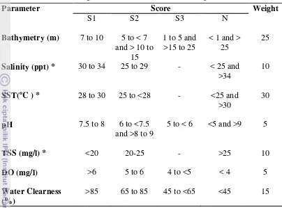
MCE is a technique combining the several criteria to determine suitability for coral reef map. A Weight linear combination (WLC) method is used to obtain suitability maps or probability map. WLC is the most often used technique for tackling spatial multi attribute decision-making. It is a multi-attribute procedure based on the concept of a weighted average. The decision maker directly assigns weights of relative importance to each attribute. A total score is then obtained for each alternative by multiplying the importance weight assigned for each attribute by the scaled value given to the alternative on that attribute, and summing the products over all attributes. When the oval scores are calculated for all the alternatives, the alternative with the highest overall score is chosen.
The WLC method can be operationalized using any GIS system having overlay capabilities. The overlay techniques allow the evaluation criterion map layers (input maps) to be aggregated to determine the composite map layer (output maps). The method can be implemented in both raster and vector GIS environments. WLC assesses the suitability of image cells by weighting and combining factor maps. WLC multiplies cell values in standardized factor maps by the corresponding factor weight, and then adds weighted values across images. Due to conditions on the weights (all positive or zero, sum equal to one), the resulting cell values are in the same range as those of the factor maps (Malczewski, 2000).
S = Wi Xi (Voogd in Wen 2008) (8)
Where: S = suitability
Wi = weight of factors i
Xi = criterion score of factors i
19
Table 7 Criteria and categorization of factor coral reef change
Parameter Score Weight
Modify: Cornelia et al. 2005 and Nugraha 2013 *
Cellular Automata (CA)
By definition, a CA is an object that has the ability to change its state based on the application of the rule that relates to the new state to its previous state and those of its neighbors (Eastman 2006). Transition area matrix and probability map for coral reef obtained from MCE model were input into CA model to attain the spatial prediction map for coral reef area. CA not only depends on the previous cell, but also on the state of the local neighborhood so the filter 5 x 5 was used in this case. Due to the use of Conway's Game of Life rules for CA, the alive or dead automata followed the criteria as mentioned below: A cell assumed as the coral reef area become alive if there are five living automata as coral reefs in the 5 x 5 neighborhood (known as the Moore neighborhood) surrounding the cell. The cell will stay alive so long as there are 4 or 5 living neighbors. Fewer than that, it dies from loneliness or it can be said that coral reef area will change to another land cover type if only one cell is assumed as the coral reef area; in addition it will compete with other resources.
CA model needs the coral reef classification map as the input that has been projected and determined at a starting time and iteration number, while the transition area files were obtained from a Markov analysis from land cover in 2002, 2007 and 2012. Furthermore, the probability map for coral reef obtained from MCE model was used as the probability map expressing the suitability of a pixel for coral reef area under several conditions.
20
Landsat Image. The second step was predicting again from 2002 until 2007 and validating by using classification map of 2007, and again from 2007 until 2012. After it had fulfilled standard Kappa Index, coral reef prediction model was created for 2022. Kappa index was used to check the accuracy of the result of coral reef prediction map. The Kappa Index for the standard agreement was >75% (very good) while that for the agreement was <40% (poor). If the model has the Kappa Index of 40%, the driving factors map for coral reef change should be repeated again based on several considerations. As suggested by Congalton et al. (1999) Kappa can be used as a measure of agreement between model predictions and reality. This research also used post-classification method as validation of distribution and the simulation result of coral reef prediction that was compared with coral reef map classification (Figure 7).
Model Validation
As mentioned previously, this stage is important in the development of any predictive model validation. Typically, the power of the model is used to predict some periods of time when the land cover conditions are known. This study has been validated by using KIA. Since KIA did not consider the spatial distribution, this research also used Post-Classification Comparison method. This analysis was done to overlay the result of prediction coral reef model 2002, 2007 and 2012 with coral reef map obtained from Landsat image and defined how many area coral cover changed.
∑ ∑
∑ (Congalton and Mead in Wassahua 2012) (9) Where:
N : the total number of cell in the matrix, r : the number of rows in the matrix Xii : the number in row i and column i
x+1 : the total observations for column i, and
x1+ : the total observations in row i
21
Figure 7 Flow chart cellular automata
4
RESULT AND DISCUSSION
Coral reef area in Barrang Lompo Island was classified by using image data with five different acquisition dates, consisting of Landsat TM 1993, 1997, and Landsat ETM+ 2002, 2007, 2012. As mentioned earlier, the five images were created from image classification using schema of habitat condition with different time series. After that, MCE process was done to obtain probability map for coral reef and followed by Markov chain analysis. Finally, spatial model for coral reef change prediction would be created with CA model and several maps as input. The result of CA model was used to predict the distribution of coral reef area in Barrang Lompo Island.
Future Trend of Coral Reef
Y
e
s
No
Kappa Validation < 75%
Kappa Validation ≥75%
Classification of coral reef (t2)
Transition area matrix (t1+ t2)
Probability Map (MCE)
M-CA Simulation
Coral reef prediction
Validation Classification of
22
Image Processing Geometric Correction
Geometric correction process was done to obtain good accuracy image position of each class in coral reef and the real world (Figure 8). Therefore, Geometric correction was performed with linear polynomial corrections to the standard type used at least 4 points (Prahasta 2008). In this study, geometric correction process was performed using 7 point GCP. The result of geometric correction shows that the average RMSE obtained from Landsat images was 0.02. It is in accordance with the standard mapping of the United States. If RMSE values are less than 0.5 pixels, this map can be said to be well corrected (Suratijaya 2010).
Figure 8 Geometric correction process
Image Classification
After image correction process had been done, Landsat Image with ISOCLASS algorithm method was classified. As mentioned in the previous chapters, the result of the classification created coral reef map based on habitat condition (live coral, dead coral, rubble, seagrass, and sand). In this study, the classification process of Landsat TM/ETM+ was done for years of 1993, 1997, 2002, 2007, and 2012 (Figure 9). The result of area calculation for coral reef changes as shown in Table 8.
Table 8. Area calculation for coral reef map 1993 to 2012
Coral Reefs Habitat
Area (ha) Percent Cover
1993 1997 2002 2007 2012 1993 1997 2002 2007 2012
Live Coral 90.07 89.35 87.52 83.01 78.86 61.61 61.12 59.87 56.78 53.94
Dead Coral 0.81 0.99 1.98 3.33 5.86 0.55 0.68 1.35 2.28 4.01
Rubble 2.34 2.7 2.7 5.86 7.48 1.60 1.85 1.85 4.01 5.12
Sand 8.44 8.87 10.1 11.57 13.03 5.77 6.07 6.91 7.91 8.91
Seagrass 44.53 44.28 43.89 42.42 40.96 30.46 30.29 30.02 29.02 28.02
Total 146.19 146.19 146.19 146.19 146.19 100 100 100 100 100
ALOS AVNIR Corrected
23
Figure 9 Coral reef classification maps with different time series from 1993 to 2012.
As mentioned in the previous chapters, the classification result was used to analyze dynamics of coral reef. Coral reef change can be seen by comparing the coral reef maps at different time series. The result of coral reefs area changing during the five dates is represented in Table 9.
Table 9 Changes in coral reef areas from 1993 to 2012 Coral
Reefs Habitat
Area Change (Ha)
1993 - 1997 1997 - 2002 2002 - 2007 2007 - 2012 1993-2012
Ha % Ha % Ha % Ha % Ha %
Live Coral -0.72 0.80 -1.83 2.05 -4.51 5.15 -4.15 5.00 -11.21 12.45
Dead Coral 0.18 18.18 0.99 50.00 1.35 40.54 2.53 43.17 5.05 86.18
Rubble 0.36 13.33 0 0.00 3.16 53.92 1.62 21.66 5.14 68.72
Sand 0.43 4.85 1.23 12.18 1.47 12.71 1.46 11.20 4.59 35.23
24
Figure 10 Coral reef changes condition in 1993 to 2012
Figure 10 shows the trend of coral reef change areas during the periods of 1993 to 2012. It can be observed that the changes from 1993 to 2012 show live coral and seagrass area decreased approximately to 11.21 ha (12.45%) and 3.57 ha (8.02%), while dead coral increased to 5.05 ha (86.18%), rubble increased 5.14 ha (68.72%), and sand increased 4.59 ha (35.23%). Live coral and seagrass areas decreased from 1993 to 2012, and the greatest decrease occurred from 2002 to 2007 covering the areas of 4.51 ha and 1.47 ha, respectively. The second greatest decreases for coral and seagrass were 4.15 ha and 1.46 ha in 2007 to 2012, respectively. While dead coral, rubble, and sand increased from 1993 to 2012. Although the extent of shallow water may change from year to year due to varying human activities and oceanography parameters, the variation in shallow water area is also likely due to classification errors (Table 10).
25
Accuracy Assessment
The result of coral reef classification maps were checked with accuracy assessment method in order to obtain the level of map accuracy. As mentioned previously, standard map accuracy was more than 70%. It can be said that these map has been classified by representing good coral reef and ground area, which were then transformed into digital paper maps. Based on confusion matrix on (Table 10) is found the OA of classification on image 2012 is 80.24%. Generally, the difference between the classification results and reality in the field is caused by water clarity and spatial resolution of satellite-derived data.
Table 10. Confusion matrix for coral reef classification in 2012
Data Classify Reference Data Row
Total
The calculation of transition probability and transition area matrix during 1993 until 2012 was done to determine the characteristic of the past and current coral reef. These processes were performed to predict the condition of next five year periods namely 2002, 2007, 2012, and 2022. This was calculated after the analysis of the coral reef change from 1993 to 2012. Types of coral reef map were computed by this method consisting of habitat conditions: coral reef, dead coral, rubble, sand, seagrass. The transition probability was used to predict coral reef condition in 2002 considering the times series trend in 1993-1997. The method of combination on the coral reef maps in two different periods resulted shown the data in Table 11.
26
The following is the transition area matrix to predict coral reef condition in 2002 considering the times series trend 1993-1997 show in Table 12.
Table 12 Transition area to predict coral reef condition in 2002 Cells in : Expected to
transition
Class 1 Class 2 Class 3 Class 4 Class 5 Class 6
Class 1 (Land) 3677 130 130 130 130 130
Class 2 (Seagrass) 0 6633 1284 0 0 0
Class 3 (Sand) 0 293 1306 0 0 0
Class 4 (Dead Coral) 6 6 6 163 6 6
Class 5 (Rubble) 0 0 111 0 369 0
Class 6 (Live Coral) 0 2 11 695 1841 13520
By using coral reef classification in 1997 as the base (t1) image while 2002 map as the later (t2) image in Markov model the transition probability matrix for prediction of coral reef condition in 2007 was obtained as shown in Table 13.
Table 13 Transition probability to predict coral reef condition in 2007 Given : Probability of
changing to :
Class 1 Class 2 Class 3 Class 4 Class 5 Class 6
Class 1 (Land) 0.8500 0.0300 0.0300 0.0300 0.0300 0.0300
Class 2 (Seagrass) 0.0000 0.8395 0.1605 0.0000 0.0000 0.0000
Class 3 (Sand) 0.0000 0.1670 0.8330 0.0000 0.0000 0.0000
Class 4 (Dead Coral) 0.0300 0.0300 0.0300 0.8500 0.0300 0.0300
Class 5 (Rubble) 0.0000 0.0000 0.2488 0.0000 0.6517 0.0000
Class 6 (Live Coral) 0.0000 0.0000 0.0363 0.0747 0.0565 0.8324
The following is the transition area matrix to predict coral reef condition in 2007 considering the times series trend 1997-2002 show in Table 14.
Table 14 Transition area to predict coral reef condition in 2007 Cells in : Expected to
transition to
Class 1 Class 2 Class 3 Class 4 Class 5 Class 6
Class 1 (Land) 3677 130 130 130 130 130
Class 2 (Seagrass) 0 6591 1260 0 0 0
Class 3 (Sand) 0 303 1514 0 0 0
Class 4 (Dead Coral) 11 11 11 316 11 11
Class 5 (Rubble) 0 0 119 48 313 0