Southern Illinois University Carbondale
OpenSIUC
Publications
Department of Plant Biology
2-1-1998
Permutation of Two-Term Local Quadrat
Variance Analysis: General Concepts for
Interpretation of Peaks
Jonathan E. Campbell
Scott B. Franklin
Southern Illinois University Carbondale
David J. Gibson
Southern Illinois University Carbondale, [email protected]
Jonathan A. Newman
Southern Illinois University Carbondale
Published in
Journal of Vegetation Science
Vol. 9, No. 1 (1998): 41-44.
This Article is brought to you for free and open access by the Department of Plant Biology at OpenSIUC. It has been accepted for inclusion in Publications by an authorized administrator of OpenSIUC. For more information, please [email protected].
Recommended Citation
Campbell, Jonathan E.; Franklin, Scott B.; Gibson, David J.; and Newman, Jonathan A., "Permutation of Two-Term Local Quadrat Variance Analysis: General Concepts for Interpretation of Peaks" (1998).Publications.Paper 7.
- Permutation of Two-Term Local Quadrat Variance Analysis - 41
Abstract. Many ecological studies use Two-Term Local Quadrat Variance Analysis (TTLQV) and its derivatives for spatial pattern analysis. Currently, rules for determining vari-ance peak significvari-ance are arbitrary. Varivari-ance peaks found at block size 1 and at > 50 % of the transect length are the only peaks whose use is explicitly prohibited. Although the use of variance peaks found at block sizes >10 % of the transect length have also been warned against, many researchers inter-pret them regardless. We show in this paper that variance peaks derived from TTLQV are subject to additional ‘rules of thumb’. Through the use of randomization and permutation analyses on real and simulated data of species abundance in contiguous plots along a single transect, we show that variance peaks found at block sizes 1, 2 and 3 occur frequently by chance and thus likely do not indicate biologically meaningful patterns. The use of multiple replicate transects decreases the probability of Type II error.
Keywords: Permutation analysis; Spatial pattern; Variance peak.
Introduction
Two-Term Local Quadrat Variance (TTLQV: Hill 1973) is one of several quadrat-based methods available to examine spatial pattern in plant and animal communi-ties. In some cases, TTLQV has been shown to detect both the scale and the intensity of spatial pattern (Usher 1975; Ludwig & Goodall 1978). Unlike earlier meth-ods, TTLQV is not restricted to detecting pattern on a scale of 2n blocks (Hill 1973; Ludwig & Reynolds
1988). However, TTLQV has some limitations. Pielou (1977) and Galiano et al. (e.g. 1987) showed that TTLQV analysis actually reports the average of the patch and gap sizes. They showed that transects with homogene-ous patch size and heterogenehomogene-ous gap size will result in variance peaks at differing block sizes. To allow for the detection of patch size per se, Dale & MacIsaac (1989) developed a method based on combinatorics that, subse-quent to quadrat-variance techniques, differentiates patch and gap sizes. In addition, Errington (1973) suggests that TTLQV will often result in block sizes that are
smaller than the actual scale of pattern when examining artificial data in which the scale of pattern is known. Dale & Blundon (1990) correct for this by stating that the true scale of pattern (B), is:
B=b+ [30b/255] + 1 (1) where b is the variance peak block size; the brackets indicate the integer part of the division. Despite these limitations, TTLQV has been useful in many studies (e.g. Greig-Smith 1979; Gibson 1988; Dale & Blundon 1990; Edwards 1994).
One problem when utilizing TTLQV is determining the meaning and significance of peaks in variance-block size graphs. This paper simply defines peaks as an increase in variance followed by a decrease in variance. While the intensity of the variance peak is important to the final interpretation of the TTLQV statistic, peak intensity is not considered here because of the problem with quantitatively determining peak significance. Al-though several researchers have attempted objective methods for evaluating the significance of peaks (e.g. χ2, Greig-Smith et al. 1963; randomization tests, Mead
1974; 95 % confidence intervals, Greig-Smith 1979; mean square, Carpenter & Chaney 1983) there is no agreed-upon method. Also, while some researchers have found that the smallest block size corresponds to some readily recognized features of the system, it has commonly been accepted that a variance peak found at the first block size is the result of sampling in quadrats that are larger than the ‘actual’ scale of pattern. In addition, Ludwig & Reynolds (1988) suggest that variances should not be analyzed for blocks >10 % of the number of quadrats when using a single transect of data. Although most researchers inter-pret block sizes up to one half of the transect length (e.g. Carpenter & Chaney 1983; Ver Hoef et al. 1989; Edwards 1994), Ludwig & Reynolds (1988) suggest that such computations lack precision. Variance peaks at interme-diate block sizes (>1 and < 10 % or half the transect length) are thought to reveal meaningful interpretations of the data.
Permutation of Two-Term Local Quadrat Variance Analysis:
General concepts for interpretation of peaks
Campbell, Jonathan E.
1*
, Franklin, Scott B.
2, Gibson, David J.
2& Newman, Jonathan A.
31USACE Waterways Experiment Station (DynTel Corporation), CEWES-ER-W, 3909 Halls Ferry Rd., Vicksburg,
MS 39180, USA; 2Department of Plant Biology, Southern Illinois University, Carbondale, IL 62901-6509, USA; 3Department of Zoology, Southern Illinois University, Carbondale, IL 62901-6501, USA;
42 Campbell, J.E. et al.
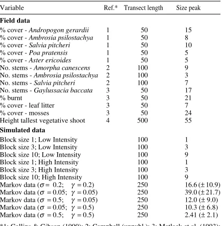
Table 1. Field and simulated data sets used in this study. Block size of first variance peak (‘Size peak’) for each of the Markov-generated data sets were averaged (± SD) over 100 runs.
Variable Ref.* Transect length Size peak
Field data
% cover - Andropogon gerardii 1 50 15
% cover - Ambrosia psilostachya 1 50 8
% cover - Salvia pitcheri 1 50 10
% cover - Poa pratensis 1 50 5
% cover - Aster ericoides 1 50 5
No. stems - Amorpha canescens 2 100 9
No. stems - Ambrosia psilostachya 2 100 3
No. stems - Salvia pitcheri 2 100 7
No. stems - Gaylussacia baccata 3 50 17
% burnt 3 50 21
% cover - leaf litter 3 50 7
% cover - mosses 3 50 24
Height tallest vegetative shoot 4 500 55 Simulated data
Block size 1; Low Intensity 100 1
Block size 3; Low Intensity 100 3
Block size 10; Low Intensity 100 9
Block size 1; High Intensity 100 1
Block size 3; High Intensity 100 3
Block size 10; High Intensity 100 9
Markov data (σ = 0.2; γ =0.2) 250 16.6 (± 10.9) Markov data (σ =0.05; γ =0.05) 250 39.0 (± 21.7) Markov data (σ =0.5; γ =0.05) 250 12.0 (± 9.0) Markov data (σ =0.05; γ = 0.5) 250 10.3 (± 6.8) Markov data (σ = 0.5; γ =0.5) 250 2.41 (± 2.1) *1: Collins & Gibson (1990); 2: Campbell (unpubl.); 3: Matlack et al. (1993); 4: Newman (unpubl.).
Permutation analyses
Permutation analyses essentially involve the ran-dom reshuffling of data points without replacement. The use of these techniques has recently increased. Longman et al. (1989) use permutation analysis to de-termine the significance of components arising in Prin-cipal Components Analysis (PCA). The primary advan-tage of this type of analysis is the reliance on a distribu-tion-free methodology. In addition, data permutations effectively eliminate the problems associated with small and/or unbalanced data sets – i.e. difficulty in testing for normality and loss of power (Potvin & Roff 1993). A final advantage of permutation analyses, assuming spa-tial variation as the sum of spaspa-tial pattern and spaspa-tially independent error, is the destruction of any auto-correlation present in the original data set (Ver Hoef et al. 1993). A disadvantage of this analysis is the rela-tively long time needed to carry out such calculations.
Our objective is to discuss peak interpretation, espe-cially the first four block sizes, when using TTLQV. To do so, we use permutation analyses to demonstrate that vari-ance peaks at block sizes 1, 2, and 3 are likely (i.e. > 88 %) to arise by chance, regardless of transect length.
Methods
Two-Term Local Quadrat Variance was applied to several real and simulated sets of transect data (Table 1).
Field data
Real data consisted of 13 variables from four sepa-rate field studies. The first two data sets were taken from tall-grass prairie studies at Konza Prairie Research Natu-ral Area, Kansas, USA. Data set 1 was a visual estimation of canopy coverage of five species in 50 contiguous 0.25 m2 quadrats (Collins & Gibson 1990). Data set 2
contained stem density counts for three species in 100 contiguous 0.25-m2 quadrats (Campbell unpubl.). Data
set 3 was taken from a study of ericaceous shrubs in the pine barrens of New Jersey coastal plains, USA (Matlack et al. 1993). Stem densities of two shrub species, cover of mosses, leaf litter, and percentage of the plot unburned in a recent fire were measured in 100 contiguous 0.25-m2
quadrats. The final data set was taken from a study of vegetation heights in a rye grass-white clover pasture in Wales (Newman unpub.). Height of the tallest vegetative shoot was recorded in 500 contiguous 5-cm2 quadrats. Simulated data
Six of the 11 simulated transects consisted of 100 contiguous quadrats. These simulated transects were created to reflect pattern at block sizes 1, 3, and 10. In addition, high and low intensity values were generated for each of the three block sizes (e.g. block size 3, low intensity: 1 1 1 0 0 0 1 1 1 0 0 0; block size 3, high intensity: 10 10 10 1 1 1 10 10 10 1 1 1). In addition, Markov chains, 250 quadrats in length, were used to create simulated transects based on five different prob-abilities of transition from patch to gap and gap to patch (Table 2). Each of the sets were run 100 × to capture variability in first peak block size results. Markov chains were employed in this study because knowledge of the expected patch and gap lengths can be maintained while a degree of stochastisity is still present within the transect. All Markovian chains used were based on a matrix of one step transition probabilities:
where σ is the probability of a transition from a gap to a patch, and γis the probability of a transition from a patch to a gap. Expected gap and patch lengths were calculated with the equation:
Permutation analysis
For the permutation analysis, we generated null model data sets from the field and simulated data to determine if spatial pattern in the data differed from patterns under a random assemblage hypothesis (Carpenter & Chaney 1983; Edwards 1994). Each permutation was analyzed with the TTLQV technique and the block size of subse-quent first peaks was recorded. 10 000 data permuta-tions, the minimum suggested by Manly (1991), were then generated for each transect. For data sets with more than one transect, permutation of individual values was made over the entire data set. The simple formula (1 – cumulative frequency) of first peak block sizes, pro-vides an empirical α-level for each block size. While this is not a true test of significance, it serves as a parsimonious determinant of whether peaks at various block sizes are justifiably interpretable as natural scale phenomena rather than stochastic occurrences. Similar Monte-Carlo procedures have been used to generate error statistics for other pattern analysis techniques (Car-penter & Chaney 1983; Ludwig & Reynolds 1988).
To ensure that the results were not merely an artifact of randomization and/or programming methodology, a second number generating method was used for the permutation analysis on all transects. This method de-termined cumulative frequency for all values along the transect. Random numbers between one and one hun-dred were then generated and matched to the cumulative frequency of the value within the data set. The value with the cumulative frequency corresponding to the random number was subsequently placed into the new data set. This was done at each point along the length of each transect. All permutations of the transect data were generated using a PASCAL program which incorpo-rated calculation of the TTLQV statistic from an earlier program written originally by A. J. Morton (Imperial College, London) and revised by T. L. Dix (University of West Florida).
Results
The sampling distribution behaved in a remarkably similar manner for all permutated transect variables.
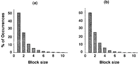
Fig. 1a shows the distribution of the ‘first peaks’ up to block size 10 for all transects. Block size 1 contains ca. 50 % of the ‘first peaks’, block size 2 contains approxi-mately one fourth, block size 3 contains approxiapproxi-mately one eighth, block size 4 contains approximately one sixteenth, and so on. This clearly shows that ‘first peaks’ recovered from permutated transect data are not rare events at block sizes 1 (≅50 %), 2 (≅25 %), or 3 (≅12 %). Variance peaks at block size 4, however, occur relatively infrequently (≅5 - 6 %), therefore ‘first peaks’ occurring at this and greater block sizes are likely due to natural scale phenomenon rather than stochastic features in the data.
These findings are echoed in the second number generating methodology (Fig. 1b). The agreement be-tween methods suggests that the phenomena is more than just an artifact of the programming language and/or the random number generation. Based on the similarity of the permutation results for all real and simulated variables and all transect lengths, results appear to be robust.
Discussion
The acceptance of spurious results is a constant threat in any study using extensive statistical calculation (see Franklin et al. 1995 for a discussion of this problem in the application of Principle Components Analysis). To aid researchers in the evaluation of their particular methodology, general guidelines are invaluable tools. Currently, TTLQV analysis has only been guided by two rules (1) do not interpret a peak at the first block size, and (2) only interpret block sizes that are less than one tenth (or one half) of the total transect length. In this paper, we suggest that TTLQV is subject to additional guidelines. In particular, block sizes 1 (α =0.5), 2 (α =0.25), and 3 (α =0.11) are not significant below their respective α-levels. In other words, block size 2 can only be considered if the examiner has a priori accepted an α-level of 0.25 or higher. Again, block size 3 can only Table 2. Transition probabilities and estimated patch and gap
sizes for data sets generated by Markovian modeling.
Data set σ γ prop g prop p E(g) E(p)
1 0.2 0.2 0.5 0.5 5 5
2 0.05 0.05 0.5 0.5 20 20
3 0.5 0.05 0.091 0.909 5 20
4 0.05 0.5 0.909 0.091 20 5
5 0.5 0.5 0.5 0.5 2 2
44 Campbell, J.E. et al.
be considered if the examiner has a priori accepted an α -level of 0.11 or higher. It is not until block size 4 (α =0.05) that the probability of accepting randomness as pattern begins to conform to the standard α-level of 0.05.
As one may expect, however, there are exceptions to this ‘rule’. In particular, block sizes 2 and 3 could be interpreted if analysis of several transects of similar data resulted in identical information. For example, the prob-ability that a local maximum in variance occurs at block size 2 on each of three independent transects reduces the possibility of a Type II error. If the random probability of a variance peak occurring at block size 2 is 0.25, then the probability of that happening on three independent transects is 0.25×0.25×0.25 = 0.016 (1.6 %) – all transects must result in exactly the same variance peak for this multiplicity of probabilities to hold true. This caveat supports the supposition that multiple transects result in more reliable data interpretation. However, multiplicity of transects does not aid in the interpreta-tion of block size 1, as actual patch may still be smaller than the quadrat size for such transects.
If one holds to the strict 10 % interpretation rule of Ludwig & Reynolds (1988), only the four block sizes in a transect of 40 quadrats should be interpreted. How-ever, our results suggest that peaks in the first three block sizes recovered from such a transect cannot be interpreted. In this case, the only interpretable peak, if it were to occur in field data analysis, would be found at block size 4. Thus, the use of single, short transects with < 40 quadrats is problematic and should be discouraged.
Acknowledgements. Partial financial support to J. E. Campbell was provided by a challenge-cost share award from the USDA-Forest Service - Shawnee National USDA-Forest, and to D. J. Gibson by NSF grants DEB-9317976 and BSR-9020426 to Kansas State University. Konza Prairie Research Natural Area is owned by the Nature Conservancy and administered by Kan-sas State University. P. Greig-Smith and S. Bartha provided constructive comments on a draft of the manuscript.
References
Carpenter, S.R. & Chaney, J.E. 1983. Scale of spatial pattern: four methods compared. Vegetatio 53: 153-160. Collins, S.L. & Gibson, D.J. 1990. Effects of fire on
commu-nity structure in tallgrass and mixed-grass prairie. In: Collins, S.L. & Wallace, L.L. (eds.) Effects of fire on tallgrass prairie ecosystems, pp. 81-98. University of Oklahoma Press, Norman, OK.
Dai, X. & van der Maarel, E. 1997. Transect-based patch size frequency analysis. J. Veg. Sci. 8: 865-872.
Dale, M.R.T. & Blundon, D.J. 1990. Quadrat variance analy-sis and pattern development during primary succession. J.
Veg. Sci. 1: 153-164.
Dale, M.R.T. & MacIsaac, D.A. 1989. New method for the analysis of spatial pattern in vegetation. J. Ecol. 77: 78-91. Edwards, G.R, Parsons, A.J., Newman, J.A. & Wright, I.A. 1996. The spatial pattern of vegetation in cut and grazed grass/white clover pastures. Grass. For. Sci. 51: 219-231. Errington, J.C. 1973. The effect of regular and random
distri-butions on the analysis of pattern. J. Ecol. 77: 78-91. Franklin, S.B., Gibson, D.J., Robertson, R.A., Pohlmann, J.T. &
Fralish, J.S. 1995. Parallel analysis: a method for determin-ing significant principal components. J. Veg. Sci. 6: 1-8. Galiano, E.F., Castro, I. & Sterling, A. 1987. A test for spatial
pattern in vegetation using a Monte-Carlo simulation. J. Ecol. 75: 915-924.
Gibson, D.J. 1988. The relationship of sheep grazing and soil heterogeneity to plant spatial patterns in a dune grassland.
J. Ecol. 76: 233-252.
Greig-Smith, P. 1979. Pattern in vegetation. J. Ecol. 67: 755-779. Greig-Smith, P., Kershaw, K.A. & Anderson, D.J. 1963. The analysis of pattern in vegetation: comment on a paper by D.W. Goodall. J. Ecol. 51: 223-229.
Hill, M.O. 1973. The intensity of spatial pattern in plant communities. J. Ecol. 61: 225-235.
Longman, R.S., Cota, A.A., Holden, R.R. & Fekken, G.C. 1989. A regression equation for the parallel analysis crite-rion in principal component analysis: mean and 95th per-centile eigenvalues. Multi. Behav. Res. 24: 59-69. Ludwig, J.A. & Goodall, D.W. 1978. A comparison of
paired-with blocked-quadrat variance methods for the analysis of spatial pattern. Vegetatio 38: 49-59.
Ludwig, J.A. & Reynolds, J.F. 1988. Statistical ecology: a primer on methods and computing. John Wiley and Sons, New York, NY.
Manly, B.F. 1991. Randomization and Monte Carlo methods in biology. Chapman Hill, London.
Matlack, G.R., Gibson, D.J. & Good, R.E. 1993. Clonal propa-gation, local disturbance, and the structure of vegetation: ericaceous shrubs in the pine barrens of New Jersey. Biol. Conserv. 63: 1-8.
Mead, R. 1974. A test for spatial pattern at several scales using data from a grid of continuous quadrats. Biometrics 30: 295-307.
Pielou, E.C. 1977. Mathematical ecology. John Wiley & Sons, New York, NY.
Potvin, C. & Roff, D.A. 1993. Distribution-free and robust statistical methods: viable alternatives to parametric sta-tistics? Ecology 74: 1617-1628.
Usher, M.B. 1975. Analysis of pattern in real and artificial plant populations. J. Ecol. 63: 569-586.
Ver Hoef, J.M., Glenn-Lewin, D.C. & Werger, M.J.A. 1989. Relationship between horizontal pattern and vertical struc-ture in a chalk grassland. Vegetatio 83: 147-155. Ver Hoef, J.M., Cressie, N.A. & Glenn-Lewin, D.C. 1993.
Spatial models for spatial statistics: some unification. J. Veg. Sci. 4: 441-452.