UNIVERSITI TEKNIKAL MALAYSIA MELAKA
IMPROVEMENT OF FRONT WHEEL STEERING SYSTEM
DUE TO SIDE WIND
This report is submitted in accordance with the requirement of the Universiti Teknikal Malaysia Melaka (UTeM) for the Bachelor of Mechanical Engineering
Technology (Automotive Technology) with Honours
By
TAN SER CHOW B071210546 920107-08-5983
DECLARATION
I hereby, declare that this thesis entitled “Improvement of front wheel steering system due to side wind” is the result of my own research except as cited in
references.
Signature : ………
Name : ………
APPROVAL
This report is submitted to the Faculty of Engineering Technology of UTeM as one of the requirements for the award of Bachelor’s Degree Mechanical Engineering
Technology (Automotive Technology) with Honours. The following are the members of supervisory committee:
……… (Supervisor)
i
ABSTRAK
Satu sistem bantuan pemandu yang dikenali sebagai stereng aktif dinilai semasa menyimulasikan pelbagai jenis acara memandu. Sistem ini merupakan sistem yang penting di dalam kenderaan itu. Tujuan utama sistem stereng adalah untuk membolehkan pemandu mengawal kenderaan secara bebas. Sistem stereng mengekalkan tayar dengan kenalan jalan. Model kenderaan kereta disimulasi oleh MATLAB / Simulink dengan 14 DOF termasuk model memandu kenderaan dan juga model pengendalian.
ii
ABSTRACT
A steering aid system called active steering is evaluated by simulating different kinds of driving events. This system is an important system in the vehicle. The main purpose of the steering system is to allow the driver control the vehicle independently. The steering system maintains the tire to the road contact. A full car vehicle model is simulated in MATLAB/Simulink with 14 DOF of equations which include the drive vehicle model and also the handling model.
The steering angle is the input of the vehicle model that should be focused on. The angle of the steering system between the tires when turning the vehicle is taken in consideration. Simulations are made on different road conditions effect and also side wind disturbances. Different values are applied to the simulation to reduce the effect of the driving events. Therefore, these simulations results do provide a better improvement to the steering system.
iii
DEDICATION
To my beloved parents
iv
ACKNOWLEDGEMENT
v
LIST OF ABBREVATIONS, SYMBOLS AND NOMENCLATURES ... x
CHAPTER 1: INTRODUCTION ... 1
1.1 Background ... 1
1.2 Problem Statement ... 2
1.3 Objectives ... 2
1.4 Scope of the study ... 2
CHAPTER 2: LITERATURE REVIEW ... 3
2.1 Introduction ... 3
2.2 Nonlinear Dynamics ... 3
2.3 Dynamic Model & Tire Model ... 5
2.4 Suspension System in MATLAB ... 8
2.5 Vehicle Stability Control ... 10
2.6 Active Front Steering System ... 12
2.7 Handling Vehicle ... 14
2.8 Four Wheel Steering System ... 17
2.9 Turning Radius ... 18
2.10 Performance of Steering System... 20
vi
CHAPTER 3: METHODOLOGY ... 24
3.1 Process Flow Chart ... 24
3.1.1 Formulation Equation ... 25
3.1.2 Equation Blocks in MATLAB & Inserting Values ... 25
3.1.3 MATLAB/Simulink ... 26
3.1.4 Result Graphs & Side Disturbances & Carsim ... 26
3.1.5 Summary ... 26
CHAPTER 4: Development of Full Vehicle Model ... 27
4.1 Introduction ... 27
4.2 Modelling Assumption ... 27
4.3 14 DOF system ... 28
4.4 Free Body Diagram ... 29
4.5 14 DOF Equation ... 31
4.5.1 Vehicle Ride Model ... 31
4.5.2 Vehicle Handling Model ... 34
4.6 Process Flow ... 37
CHAPTER 5: Discussion ... 52
5.1 Introduction ... 52
5.2 Stability Test ... 52
5.3 Validation Response of 14 DOF Vehicle Model with an Instrumented Experimental Vehicle ... 53
5.3.1 Lateral Acceleration ... 54
5.3.2 Longitudinal Acceleration ... 56
5.3.3 Yaw Control ... 59
CHAPTER 6: Conclusion ... 62
vii
LIST OF TABLES
Table 2.1: Fixed Parameters of Full Car Model ... 8
Table 2.2: Vehicle Parameters ... 15
Table 2.3: Comparison for Two Wheel Steer and Four Wheel Steer ... 18
Table 2.4: Comparison of Four Wheels and Two Wheel Steering System ... 19
Table 2.5: Application and Safety Function of Hardware and Users... 22
Table 5.1: Data Lateral Acceleration versus Time ... 55
Table 5.2: Data Longitudinal Acceleration versus Time ... 57
viii
LIST OF FIGURES
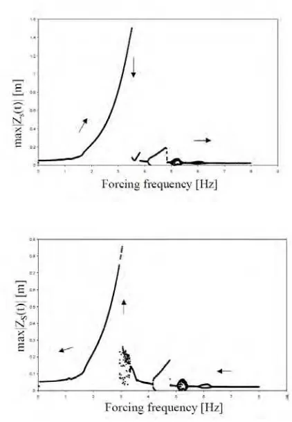
Figure 2.1: Frequency Response Diagrams when the Forcing Frequency f is slowly
Increased and Decreased ... 4
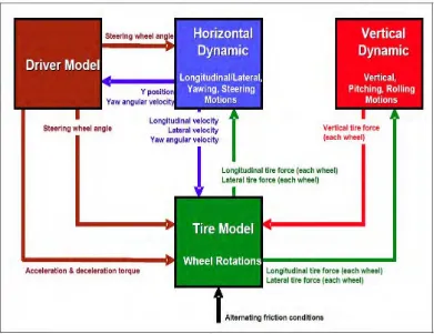
Figure 2.2: Modular Architecture of Vehicle Model ... 6
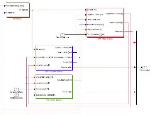
Figure 2.3: Modular Vehicle Model in MATLAB/Simulink ... 7
Figure 2.4: Sprung Mass Displacement (ZCG) vs. Time in Simulink Model ... 9
Figure 2.5: Sprung Mass Displacement (ZCG) vs. Time using Analytical solutions (State Space)... 9
Figure 2.6: Displacement vs Time for K=25000, C=4000 ... 10
Figure 2.7: 7 DOF Complex Model, Dashed Line: Simplified Model ... 11
Figure 2.8: Schematic view of AFS system ... 12
Figure 2.9: (a) Steering Wheel Angle and Front Wheel Angle of Slalom Test; (b) Pylon Markers of Slalom Test... 14
Figure 2.10: Simulated Lateral Acceleration ... 16
Figure 2.11: Simulated Roll Angle ... 16
Figure 2.12: Designed CATIA Model ... 17
Figure 2.13: Power Steering System as Part of the Vehicle’s Close Loop ... 21
Figure 2.14: Slalom Ride (Cones Distance: 16m and Vehicle Velocity 50 kph) ... 23
Figure 3.1: Flow Chart Part 1... 24
Figure 3.2: Flow Chart Part 2... 25
Figure 4.1: 14 DOF Full Vehicle Model ... 29
Figure 4.2: Vehicle Handling Model ... 30
Figure 4.3: Full Car Vehicle Model ... 31
Figure 4.4: Launched Carsim Software ... 37
Figure 4.5: Vehicle Configuration Sedan E-Class Model Selected ... 37
Figure 4.6: Procedure Crosswind Test Selected ... 38
Figure 4.7: Result 3 deg. Azimuth. Veth. Ref. Selected to Animate ... 38
Figure 4.8: Graph Steering Wheel Angle Selected ... 39
Figure 4.9: Graph Lateral Acceleration of CG’s Selected ... 39
Figure 4.10: Graph Yaw Angle of Sprung Masses Selected... 40
ix
Figure 4.12: Graph Longitudinal Acceleration of CG’s Selected ... 41
Figure 4.13: Graph Roll Angle of Sprung Masses Selected ... 41
Figure 4.14: Run Math Model & Animated ... 42
Figure 4.15: Lateral Side Wind Tested ... 42
Figure 4.16: Graph Yaw Angle Vs Time Plotted by Carsim ... 43
Figure 4.17: Graph Lateral Acceleration Vs Time Plotted by Carsim... 43
Figure 4.18: Longitudinal Acceleration Vs Time Plotted by Carsim ... 44
Figure 4.19: Data Graph by WordPad ... 44
Figure 4.20: Data Transferred to Microsoft Excel ... 45
Figure 4.21: Launched Matlab Software... 45
Figure 4.22: Parameter of Vehicle Model E-Class ... 46
Figure 4.23: Parameter is transferred from Carsim ... 46
Figure 4.24: Run the Simulation ... 47
Figure 4.25: Graph Yaw Vs Time Plotted by Matlab ... 47
Figure 4.26: Graph Lateral Acceleration Vs Time Plotted by Matlab ... 48
Figure 4.27: Graph Longitudinal Acceleration Vs Time Plotted by Matlab ... 48
Figure 4.28: Data Compared for Validation Purpose ... 49
Figure 4.29: Data Imported to Vehicle Model ... 49
Figure 4.30: Validation Graph of Yaw Vs Time ... 50
Figure 4.31: Validation Graph of Lateral Acceleration Vs Time ... 50
Figure 4.32: Validation Graph of Longitudinal Acceleration Vs Time ... 51
Figure 5.1 Validation of Lateral Acceleration Vs Time... 54
Figure 5.2: Validation of Longitudinal Acceleration Vs Time ... 56
x
LIST OF ABBREVATIONS, SYMBOLS AND
NOMENCLATURES
AFS - Active Front Steering
CG - Centre Gravity
DOF - Degree of Freedom
HSRI - Human Services Research Institute
ISO - International Organization for Standardization
MATLAB - Matrix Laboratory
RPM - Rotation per Minute
RAM - Random Access Memory
ROM - Read-only Memory
SBW - Steer-by-Wire
VSC - Vehicle Stability Control
F
fl Suspension force at thefront left corner
Z
u,fl Front left unsprung masses displacementF
fr Suspension force at thefront right corner
Z
u,rr Rear right unsprung masses displacementF
rl Suspension force at therear left corner
Z
u,rl Rear left unsprung masses displacementF
rr Suspension force at therear right corner u,fr Front right unsprung masses velocity
xi
K
s,fl Front left suspensionspring stiffness
a
Distance between front of vehile and C.G. of sprung massK
s,fr Front right suspensionspring stiffness
b
Distance between rear of vehicle and C.G. of sprung massKs,rr Rear right suspension
spring stiffness Pitch angle at body centre of gravity Ks,rl Rear left suspension
spring stiffness Roll angle at body centre of gravity Cs,fr Front right suspension
damping
Z
s,fl Front left sprung mass displacement Cs,fl Front left suspensiondamping
Z
s,fr Front right sprung mass displacement Cs,rr Rear right suspensiondamping
Z
s,rl Rear left sprung mass displacement Cs,rl Rear left suspensiondamping
Z
s,rl Rear left sprung mass displacement Zu,fr Front right unsprungmasses displacement
Z
s,rr Rear right sprung mass displacement Pitch rate at bodycentre of gravity
u,fr Front right unsprung
masses acceleration
Zs Sprung mass
xii
r Rear side slip angle
Wheel base of sprung
sx The moments of inertia
of the sprung mass around the x-axes
sy The moment of inertia
1
CHAPTER 1
INTRODUCTION
1.1 Background
In an age of advanced technology, automobile was a life’s necessities for everyone. It also acts as a transportation to travel for a distance no matter a short or long journey. Therefore, automobile had become more and more convenience nowadays. In this competitive field, vehicle must be improved in comfort and safety. By doing so, development of vehicles should be done to ensure new technology is implanted into the driving system to enhance driver pleasure.
A vehicle consists of many systems to maintain each of the vehicle parts function well. The steering system acts as one of the important system in the vehicle. For commonly known, steering system used to drive the vehicle to different directions which control by the driver alone. Then, the steering system also provided the driver a road feel feedback when the vehicle drove through an uneven surface or facing the wind disturbances. The main purpose of the steering system is to make contact between the tire and the road surfaces. Therefore, concentrations were mainly focus on the tire life of the vehicle to achieve better angle of the steering system. Furthermore, the driver can turned their vehicle with minimum effort by the help of the steering system which is not so easy to control.
2
1.2 Problem Statement
The problem in this project is the side wind disturbances. This problem could contribute to vehicle stability. Therefore, this project focused on the improvement of the front steering system. This study wills focused and highlighted these problems that become challenges to complete the task. Therefore, simulations between the Matlab model and Carsim actual model which both consists of 14 DOF equations are made to improve the front steering system.
1.3 Objectives
The main objective of this project is to focus on the design and development of mathematical equations, apply them to the MATLAB Simulink and make some modification on controller design.
1.4 Scope of the study
Scopes of the study are listed as follows:
i) Identifying the effects of the vehicle riding.
ii) Developed mathematical equation with 14 Degree Of Freedom vehicle model.
iii) Produce a Simulink diagram by using the MATLAB software and compare with Carsim.
3
CHAPTER 2
LITERATURE REVIEW
2.1 Introduction
For further process of this research project, literature review made an important key of it. Literature survey in various fields, such as active steering system, steering control, handling, vehicle modelling and parameters estimation is carried out to establish the state of the art.
2.2 Nonlinear Dynamics
First, the dynamic behaviour of a nonlinear seven degrees-of-freedom ground vehicle model is examined. The nonlinearity occurs due to suspension dampers and springs. The disturbances from the road are assumed to be sinusoid and the time delay between the disturbances is also considered. Numerical results show that the responses of the vehicle model could be chaotic. Using bifurcation phenomenon, the chaotic motion is detected and confirmed with the Poincare’ maps. The results can be applicable in dynamic design of a vehicle. [Hajikarami et al, 2009]
4 Because of high nonlinearities of differential equations in the full car model, the dynamic response of the system is studied numerically using the forth order Runge-Kuntta algorithm provided by MATLAB.
The frequency responses diagrams are obtained by plotting the amplitude of the oscillating system versus the frequency of the excitation. This are used to analyse the dynamics of a system. Bifurcation is the phenomenon of sudden change in the motion as a parameter is varied. Therefore, the parameter values at which they occur are called bifurcation points. Poincare’ maps were one of the instruments to analyse the dynamic system.
In the interval of 4.96< <5.47 Hz, there are two unstable regions caused by the increasing in frequency, =3.08Hz as a huge jump and a small jump which was =3.18Hz is observed from the figure 2.1. = 4.76 Hz and = 3.07 Hz is observed for the decreasing frequency. Besides, 4.99< <5.41 Hz and 2.97< < 3.55 Hz was the unstable region.
Figure 2.1: Frequency Response Diagrams when the Forcing Frequency f is slowly
5 As conclusion from the frequency response diagrams, the number of jumps and unstable regions of the response were focused. The result of increasing frequency is different from those for decreasing frequency. This was an ordinary phenomenon for nonlinear problems but the phenomenon was not observed in the study of two or four DOF vehicle model.
2.3 Dynamic Model & Tire Model
Most of reference models for chassis controls usually have low level degree of freedom like a bicycle model. However, these models include some different value in real vehicle motion and have a difficulty to adapt new technology. In addition, it is not good for real time that very high degree of freedom like multi-body dynamic analysis programs because of their long solving time. So, I developed adaptive full vehicle dynamic model that has 14 degree of freedom with theoretical equations and experimental data. [Lee et al, 2008]
This paper studies the technology for a thesis of a vehicle dynamics model based on a full car model with 14 DOF (Degree of Freedom). MATLAB was done on the 14 DOF full vehicle models which consist of horizontal direction and vertical direction. 14 DOF model consider of whole direction of the full car vehicle model. The time used in this software was less compared to commercial program. Therefore, a more accurate result can be obtained.
6
7
Figure 2.3: Modular Vehicle Model in MATLAB/Simulink
8
2.4 Suspension System in MATLAB
Suspension system design is a challenging task for the automobile designers in view of multiple control parameters, complex objectives and stochastic disturbances. For vehicle, it is always challenging to maintain simultaneously a high standard of ride comfort, vehicle handling under all driving conditions. The objective of this paper is to develop a MATLAB/SIMULINK model of a full car to analyse the ride comfort and matrix are to be developed and validation of Simulink model with analytical solution of state space matrix is to be done elaborately on this paper. [Mitra et al, 2008]
In this research, mathematical modelling was taken in measure using seven degree of freedom model of the full car for passive system. There were mathematical equation formed which include sprung mass and also unsprung mass of a full model vehicle. Next, the equation was tested with MATLAB/SIMULINK to obtain the result from the graphs. From the result obtained, vehicle body acceleration was high at velocity of 10kmph. Therefore, the effect of bump of same amplitude had no effect on pitch angle and roll angle of the vehicle.
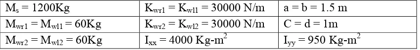
The fixed parameters mentioned in various research papers are taken for the simulation study. Suspension spring stiffness were considering 55000 N/m, 25000 N/m and damping coefficient 4000 N-s/m, 1000 N-s/m respectively. The combination of stiffness and damping coefficient were studied in simulation.
Table 2.1: Fixed Parameters of Full Car Model
Ms = 1200Kg Kwr1 = Kwl1 = 30000 N/m a = b = 1.5 m
Mwr1 = Mwl1= 60Kg Kwr2 = Kwl2 = 30000 N/m C = d = 1m
9
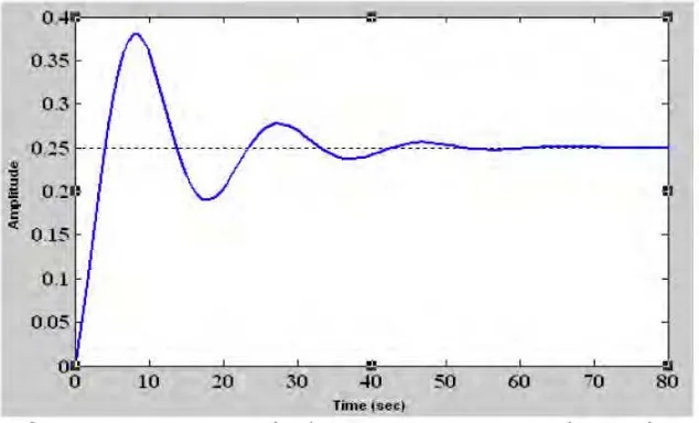
Figure 2.4: Sprung Mass Displacement (ZCG) vs. Time in Simulink Model
Figure 2.5: Sprung Mass Displacement (ZCG) vs. Time using Analytical solutions
(State Space)
This validated simulation model was ride comfort and road holding for different standard road profiles. As results, the speed range of 5 to 10kmph must be an optimum speed to cross the bump without affecting the Human tolerance zone of 0.315 m/s2 to 0.625 m/s2 as per ISO standard. There was no effect on pitch angle and