THEORETICAL ANALYSIS OF AN IMPROVED COVARIANCE MATRIX ESTIMATOR IN
NON-GAUSSIAN NOISE
F. Pascal
123, P. Forster
2, J-P. Ovarlez
1, P. Larzabal
3.
1
ONERA, Chemin de la Huni`ere, F-91761 Palaiseau Cedex, France
2
GEA, 1 Chemin Desvalli`eres, F-92410 Ville d’Avray, France
3
ENS Cachan, 61 Avenue du Pr´esident Wilson, F-94235 Cachan Cedex, France
Email : [email protected], [email protected], [email protected],
[email protected]
ABSTRACT
This paper presents a detailed theoretical analysis of a recently introduced covariance matrix estimator, called the Fixed Point Es-timate (FPE). It plays a significant role in radar detection applica-tions. This estimate is provided by the Maximum Likelihood Es-timation (MLE) theory when the non-Gaussian noise is modelled as a Spherically Invariant Random Process (SIRP). We study in details its properties: existence, uniqueness, unbiasedness, consis-tency and asymptotic distribution. We propose also an algorithm for its computation and prove the convergence of this numerical procedure. These results will allow to study the performance anal-ysis of the adaptive CFAR radar detectors (GLRT-LQ, BORD,...).
1. PROBLEM STATEMENT AND BACKGROUND
Non-Gaussian noise characterization has gained many interests sin-ce experimental radar clutter measurements showed that these data are correctly described by non-Gaussian statistical models. One of the most tractable and elegant non-Gaussian model comes from the so-calledSpherically Invariant Random Process(SIRP) theory. A SIRP is the product of a Gaussian random process - calledspeckle
- with a non-negative random variable - calledtexture. This model leads to many results [1, 2, 3, 4].
The basic problem of detecting a complex signal corrupted by an additive SIRP noisecin am-dimensional complex vectory al-lowed to build several Generalized Likelihood Ratio Tests like the GLRT-Linear Quadratic (GLRT-LQ) in [1, 2] or the Bayesian Op-timum Radar Detector (BORD) in [3, 4].
Let us recall some SIRP theory results. A noise modelled as a SIRP is a non-homogeneous Gaussian process with random power. More precisely, a SIRP [5] is the product of a positive ran-dom variableτ (texture) and am-dimensional independent com-plex Gaussian vectorx(speckle) with zero mean covariance matrix M=E(xx†)with normalization tr(M) =m, where†denotes the conjugate transpose operator :
c=√τx.
The SIRP PDF expression is:
pm(c) = Z +∞
0
gm(c, τ)p(τ)dτ , (1)
where
gm(c, τ) = 1
(π τ)m|M| exp
„ −c
†
M−1c τ
«
. (2)
In many problems, non-Gaussian noise can be characterized by SIRPs but the covariance matrix Mis generally not known and an estimateMb is required. Obviously, it has to satisfy the M-normalization: tr(Mb) =m.
In the literature [6, 7], the Normalized Sample Covariance Ma-trix Estimate (NSCME) defined as follows is usually used:
b
MNSCM E=m
N N
X
i=1
cic†i
c†ici
!
= m
N N
X
i=1
xix†i
x†ixi
!
, (3)
where1≤i≤N ,ci=√τixiarem-dimensional indepen-dent complex SIRP vectors andxiarem-dimensional independent complex Gaussian vectors with zero mean and normalized covari-ance matrixM.
This estimate is remarkably independent of the texture statis-tics. However, despite of this interesting property, the NSCME (3) suffers the following drawbacks:
• it is a biased estimate;
• the resulting adaptive Generalized Likelihood Ratio (GLR) is not independent of matrixMcharacteristics.
In the next sections, we propose to introduce and analyze an improved estimator ofM: the FPE estimator.
2. THE FIXED POINT ESTIMATORMF Pb
Conte and Gini in [8, 9] have shown that the Maximum Likelihood estimatorMb ofMis a solution of the following equation:
b
M=m
N N
X
i=1
cic†i
c†iMb−1ci
!
. (4)
Let functionfbe defined as:
f(Mb) = m
N N
X
i=1
cic†i
c†iMb−1ci
!
, (5)
and notice thatfcan be rewritten as follows, which shows thatMb is also texture statistics independent:
f(Mb) = m
N N
X
i=1
xix†i
x†iMb−1xi
!
. (6)
Theorem 1
1. the functionfadmits a single fixed point, calledMf pb , which verifies
f(Mf pb ) =Mf p.b (7)
2. Let us consider the recurrence relation
b
Mt+1= m tr“f(Mtb )”
f(Mtb ) (8)
ThenMtb −−−→ t→∞ Mf pb .
The point one of the theorem shows that the Maximum Like-lihood estimateMf pb exists and is unique.
1 10 40 80
10−16
10−14
10−12
10−10
10−8
10−6
10−4
10−2
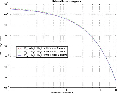
100 Relative Error convergence
Number of Iterations
||M
t+1
−
M
t
|| / ||M
t
||
||Mt+1− Mt|| / ||Mt|| for the matrix 2−norm
||Mt+1− Mt|| / ||Mt|| for the matrix 1−norm ||Mt+1− Mt|| / ||Mt|| for the Frobenius norm
Fig. 1. Illustration of the convergence to the fixed point.
Figure 1 illustrates the second point of the above theorem. On this figure, the relative errorf(Mtb )−Mtb /Mtb has been plot-ted versustwith initial valueMb0=MNSCM Eb (3).
Other simulations have been performed with different initial valuesMb0(ex : sample Gaussian covariance estimate, matrix with
uniform PDF, deterministic Toeplitz matrix), each of them con-ducting to the same value with an extremely fast convergence :
f(Mtb )−Mtb −−−→ t→∞ 0
ButMf pb is only given in (7) as an implicit function of the data: there is no closed form expression forMf pb . So, it is a significant feature to characterizeMf pb by its properties. The statistical prop-erties have never been investigated. The purpose of this paper is
to fill these gaps by establishing the bias, the consistency and the asymptotic distribution of this random matrix: this is the aim of the next section.
3. MF Pb PROPERTIES
In order to simplify the notations in the proofs, let us define the following quantities:
• Mb =Mf pb ;
• ∆=M−1/2M Mb −1/2−ImwhereImis them×m iden-tity matrix;
• X =vec(∆)whereXis the vector containing all the el-ements of∆and vec denotes the operator which reshapes them×nmatrix elements into amncolumn vector;
• ⊤denotes the transpose operator.
3.1. Bias and consistency
Proposition 1 Mf pb is unbiased and it is a consistent estimator.
Proof 1 This proof will appear in a forthcoming journal paper. It is too long to fit here and we decided to detail the proof of the next proposition.
3.2. Mf pb covariance matrix
Proposition 2 We have the following original results with the above notations:
1. √N
»
Re(X)
Im(X) –
law
−−−−−→N→+∞ N`02m2,C
´
, where−−→law
rep-resents the convergence in distribution;
2. NE`XX⊤´= „
m+ 1
m
«2
C1where
C1=
m m+ 1
„
P− 1
mvec(Im)vec(Im)
⊤
« ; (9)
3. NE`XX†´= „
m+ 1
m
«2
C2where
C2=
m m+ 1
„
Im2−
1
mvec(Im)vec(Im)
⊤
«
. (10)
Notice thatC, which is the covariance matrix of
»
Re(X)
Im(X) –
,
is fully characterized by the two quantitiesE`XX⊤´andE`XX†´.
Proof 2 First, let us defineMb =M+∆1. Notice that
∆1=M1/2∆M1/2. (11) For largeN,∆1≃0m×mbecause of theMb consistency.
We can write
ForNlarge enough, this implies that:
b plex vectors with identity covariance matrix. Then,
M−1/2∆1M−1/2≃
or equivalently using expression (11),
∆≃ mN
We obtain at the first order, for large N,
∆≃ mN
To find the explicit expression of∆in terms of data, the above expression can be reorganized as:
∆−Nm
To solve thism2-system, the above equation has to be rewrit-ten as:
Notice that the vec operator reorganizes the matrix elements as follows: ifH =`hij´1
≤i,j≤m and vec(H) = (vk)1≤k≤m2,
thenhij=vkfork= (j−1)m+i.
Let us set in equation (18):
A=vec m
Using the Central Limit Theorem (CLT), the right hand side of equation (18) satisfies:
√
whereGis the covariance matrix of
»
Re(A)
Im(A) –
,
whileBat the left hand side, by the Strong Law of Large Num-bers (SLLN), has the following property:
B−−−−−→a.s.
Thus, from standard probability convergence considerations, we obtain the first point of proposition 2. Moreover, for largeN, we have the following equations:
E`XX⊤´ = C2−1E`AA⊤´C−21
E`XX†´ = C−21E`AA†´C−21 . (22)
Let us now turn to the closed form expression of C2.
C2=Im2−mE
are independent variables, withrj∼χ2(2)andθj
∼ U([0,2π]).
Thus, with the above notations, we have:
Ekl=E and only if
1. p=q=p′=q′
which is equivalent to:
2. k=p+m(p−1), l=p′+m(p′
−1) andp=p′
, i.e.
k=l
3. k=p+m(q−1), l=p+m(q−1) andp=q.
Finally, the non zero elements of the matrixEare:
1. Ep+m(p−1),p+m(p−1)=E
r2
p
`Pm j=1rj
´2
!
= 2
m(m+ 1)
2. Ep+m(p−1),p′+m(p′−1)=E
rprp′
`Pm j=1rj
´2
!
= 1
m(m+ 1)
3. Ep+m(q−1),p+m(q−1)=E
rprq
`Pm j=1rj
´2
!
= 1
m(m+ 1)
In summary, we obtain the closed form expression ofC2given by (10). In a similar way, we have derived the following results:
• C1=
m m+ 1
„
P− 1
mvec(Im)vec(Im)
⊤
«
wherePis the
m2
×m2nilpotent matrix defined as follows:
Pij= 0 and for 1≤p, p′ ≤m:
- Pp+m(p−1), p+m(p−1)= 1, - Pp+m(p′−1), p′+m(p−1)= 1,
• NE`AA⊤´=C1andNE`AA†´=C2.
4. APPLICATIONS
In radar detection, the following test is used to detect, in an m-vector observationz, a complex known signalswhose Doppler characteristics are represented here by its steering vectorp:
ˆ
Λ(Mb) = |p
†b
M−1z|2
(p†Mb−1p)(z†Mb−1z)
H1 ≷
H0
λ . (24)
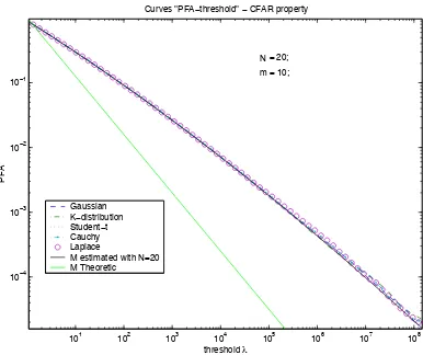
In a previous paper [10], we have derived the closed form expres-sion of the relation between the Probability of False Alarm (PFA) and the detection thresholdλ, under Gaussian noise assumption and forMb equal to the sample covariance matrix (Wishart dis-tributed).
As illustrated on the Figure 2, results obtained in this paper allowed us to show that the previous relation is surprisingly still valid under any SIRP noise and forMb equal to the FPE. Indeed, the covariance matrix of the Wishart matrix (not done in this pa-per) is the same near to a multiplicative scalar factor as the FPE covariance matrix established in this paper. Then, the asymptotic behavior of the previous estimates is the same near to a multiplica-tive scalar factor.
5. CONCLUSIONS AND OUTLOOK
We have established in this paper the theoretical statistical prop-erties (unbiasedness, consistency, asymptotic distribution) of the MLE SIRP kernel covariance matrix estimate. Simulation results have confirmed the validity of this work.
These properties will be of practical use in radar detection for establishing the statistics of the GLRT-LQ or BORD radar detec-tors. These adaptive detectors built with the FPE will have the fol-lowing significant feature: they will be SIRP-CFAR (independent of the texture statistics as well as the structure of the covariance matrixMof the SIRP gaussian kernel).
101 102
103 104
105 106
107 108 10−4
10−3 10−2 10−1
threshold λ
PFA
Curves "PFA−threshold" − CFAR property
Gaussian K−distribution Student−t Cauchy Laplace M estimated with N=20 M Theoretic
N = 20; m = 10;
Fig. 2. Relation ”PFA-threshold” for different SIRP noises
6. REFERENCES
[1] E. CONTE, M. LOPS ANDG. RICCI,”Asymptotically Op-timum Radar Detection in Compound-Gaussian Clutter”,
IEEE Trans.-AES,31(2) (April 1995), 617-625.
[2] F. GINI, ”Sub-Optimum Coherent Radar Detection in a Mixture of K-Distributed and Gaussian Clutter”, IEE Proc.Radar, Sonar Navig,144(1) (February 1997), 39-48.
[3] E. JAY, J.P. OVARLEZ, D. DECLERCQ AND P. DUVAUT,
”BORD : Bayesian Optimum Radar Detector”,Signal Pro-cessing,83(6) (June 2003), 1151-1162
[4] E. JAY,”D´etection en Environnement non-Gaussien”,Ph.D. Thesis, University of Cergy-Pontoise / ONERA, France, June 2002.
[5] K. YAO”A Representation Theorem and its Applications to Spherically Invariant Random Processes”,IEEE Trans.-IT, 19(5)(September 1973), 600-608.
[6] E. CONTE, M. LOPS, G. RICCI,”Adaptive Radar Detection in Compound-Gaussian Clutter”, Proc. of the European Sig-nal processing Conf., September 1994, Edinburgh, Scotland.
[7] F. GINI, M.V. GRECO, AND L. VERRAZZANI, ”Detec-tion Problem in Mixed Clutter Environment as a Gaussian Problem by Adaptive Pre-Processing, Electronics Letters, 31(14)(July 1995), 1189-1190.
[8] E. CONTE, A. DEMAIO ANDG. RICCI,”Recursive Esti-mation of the Covariance Matrix of a Compound-Gaussian Process and Its Application to Adaptive CFAR Detection”,
IEEE Trans.-SP,50(8)(August 2002), 1908-1915.
[9] F. GINI, M. GRECO, ”Covariance Matrix Estimation for CFAR Detection in Correlated Heavy Tailed Clutter”,Signal Processing, special section on Signal Processing with Heavy Tailed Distributions,82(12)(December 2002), 1847-1859.
[10] F. PASCAL, J.P. OVARLEZ, P. FORSTER AND P. LARZA