Dependent Selling Rate
Wahyudi Sutopo†
Department of Industrial Engineering, Bandung Institute of Technology Jalan Ganesa 10, Bandung 40132, INDONESIA
Department of Industrial Engineering, University of Sebelas Maret Jalan Ir. Sutami No. 36 A, Surakarta 57136, INDONESIA. E-mail: [email protected] or [email protected]
Senator Nur Bahagia
Department of Industrial Engineering, Bandung Institute of Technology Jalan Ganesa 10, Bandung 40132, INDONESIA
Email: [email protected]
Abstract. Economic order quantity (EOQ) is one of the most important inventory policy that have to be decided in managing an inventory system. The problem addressed in this paper concerns with the decision of the optimal replenishment time for ordering an EOQ to a supplier. This Model is captured the affect of stock dependent selling rate and varying price. We developed an inventory model under varying of demand-deterioration-price of commodity when the relationship of supplier-grocery-consumer at stochastic environment. The replenishment assumed instantaneous with zero lead time. The commodity will decay of quality according to the original condition with randomize characteristics. First, the model is addressed to solve a problem phenomenon how long is the optimum length of cycle time. Then, an EOQ of commodity to be ordered by will be determined by model. To solve this problem, the first step is developed a mathematical model based on reference’s model, and then solve the model analytically. Finally, an inventory model for deteriorating commodity under stock dependent selling rate and considering selling price was derived by this research.
Keywords: deterioration commodity, expected profit, optimal replenishment time stock dependent selling rate.
1.INTRODUCTION
The deteriorating commodity is defined as a commodity with decay or loss of quality marginal value that results in the decreasing usefulness from the original condition (Nahmias, 1982; Dave, 1991, and Raafat, 1991). Firms selling commodity whose quality level deteriorates over time often face difficult decisions when unsold inventory remains. Since the leftover commodity is often perceived to be of lower quality than the new commodity, carrying it over offers the firm a second selling opportunity and also reduced selling price. In this case, firms should choose optimal strategy as trade of order quantity from supplier and selling price down policy as impact of deterioration rate.
Unfortunately, some commodities, like fresh foods, vegetables, fruits and cooking spices, will be perishable or spoiled when the lifetime is over. In contrast, Grosser faces a market potential with a stochastic environment for instant cost per unit, life time and demand of commodity. They should obtain inventory policy to maximize their profit.
A survey of literature on inventory models for deteriorating items was given by Raafat (1991) and
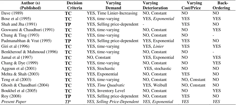
Nahmials (1992). This research is started with concerning a variety of inventory models from previous researches that consider the effect of deterioration and perishable with time dependent. The following scheme is used to categorize the various models for instant: (i) decision criteria: total cost or total profit; (2) consider varying demand; (3) consider deterioration varying, and consider cost/price varying (Table 1).
Table 1: Summary of the related research
Author (s) (Published)
Decision Criteria
Varying Demand
Varying Deterioration
Varying Cost/Price
Back- Ordering
Dave (1989) TC YES, Time Linier-Increasing NO, Constant NO NO
Bose et al (1995) TC YES, time-varying YES, Exponential YES YES
Shah and Jha (1991) TP YES, Selling price-dependent - YES NO
Goswami & Chaudhuri (1991) TC YES, time-varying NO, Constant NO YES
Chung & Ting (1993) TC YES, time-varying NO, Constant NO -
Padmanabhan & Vrat (1995) TP YES, Selling price-dependent YES, Exponential YES NO
Giri et al (1996) TC YES, time-varying YES, Linier YES YES
Benkherouf & Mahmoud (1996) TC YES, time-varying NO, Constant NO -
Jamal et al (1997) TC NO, Constant YES, Exponential NO YES
Chang & Dye (1999) TC YES, time-varying NO, Constant NO YES
Aggoun et al (2001) TC YES, Stochastic YES, stochastic NO NO
Mehta & Shah (2003) TC YES, Exponential NO, Constant YES NO
Teng et al (2003) TC YES, time-varying NO, Constant NO, Constant NO
Ghosh & Chaudhuri (2004) TC YES, Time Quadratic YES, Weibull NO, Constant NO
Boukhel et al (2005) TC YES, Inventory Level NO, Constant NO YES
Roy (2008) TP YES, Selling price-dependent NO, Constant YES NO
Present Paper TP YES, Selling Price-Dependent YES, Exponential YES YES
In most previous models, integration among supply depend on selling price with price policy in stochastic market environment was not conducted yet. In most models do not considered selling price. Then, the minimize total cost were used as decision criteria. Shah & Jha (1991) have started to developing inventory model with maximize profit as decision criterion, however the model do not be related to the impact of deterioration rate. Aggoun et al (2001) have conducted to integrate among deterioration with inventory level in one particular market environment which is stochastic. However, they do not considering cost or price varying yet as the impact of deterioration rate.
In the present paper, we have developed an inventory model for deteriorating commodity under stock dependent selling rate and considering selling price. The performance criterion of this model is to maximize profit by simultaneously determining the selling price.
2. THE PROBLEM FORMULATION
The novelty we will be taking into consideration in this research is developed an inventory model under varying of demand-deterioration-price of commodity when the relationship of supplier-grocery-consumer at stochastic environment. First, the model is addressed to solve a problem phenomenon how long is the optimum length of cycle time. Then, an EOQ of commodity to be ordered by will be determined by model during the length of cycle time to get maximum profit. The framework of a stochastic inventory model for deteriorating commodity was shown in Figure 1.
Figure 1 is described the characteristic on natural of inventory system. It was depicted by the following:
(i) this system is constructed by single supplier, single grosser and many consumers;
(ii) the item is a single commodity. Each commodity will decay of quality according to the original condition with randomize characteristics; and
(iii) all stock outs (shortages) are lost and not recovered, and
[image:2.595.326.548.345.589.2](iv) the excess stocks is expired and no value.
Figure 1: Framework of an inventory model
Mathematical Abbreviations and Symbols
The mathematical model is derived with the following assumptions and notations:
(1). In a cycle of planning horizon, the costs of the model is as follows:
i).
a fixed ordering cost,A
;ii).
a holding cost per unit in stock per unit of time that proportional with price and time,h
;iii).
a shortage cost per unit of item per unit of tim e,k
iv).
a purchase cost per unit of item,p
(2). The replenishment assumed instantaneous (uniform) with zero lead time,
L
= 0.(3). The single commodity deteriorates with rates,
j, a specific density function.(4).
I
(t), is the inventory level at timet
.(5).
T
D, is total demand where the demand rate (the selling rate),D
(t), at timet
, that may occur as long asT
, depends on the change in inventory level,I
(t) and parameter of stock dependent selling,b
is assumed D(t)ab.I(t).(6). The excess of stocks,
Q
u, is expired and no value. (7). Selling price,P
,Decision Variables :
R
T
: is total revenue from selling a single commodity.C
T
: is total of Inventory costP
T
: is total profit that calculated byT
R-T
C.T
: is the length of the cycle time.EOQ :
The quantity of commodity to be ordered by grosser is an economic order quantity,
*
Q
Q
s
during the length of the cycle time.3. THE MATHEMATICAL MODEL
We first analyze the model of Aggoun el al (2001) as reference and then develop a new stochastic inventory model based on periodic review system (P Model), Aggoun et al (2001) dan Shah & Jha (1991). The mathematical model formulation is developed with the following steps:
(1). total of inventory cost
The total of inventory costs is consists the total of purchase cost (
O
b), ordering cost (O
p); holding cost (O
s), shortage cost (O
k) and excess cost (O
u). In consequence the total cost in this inventory system can be written as:u k s p b
c
O
O
O
O
O
T
(1)(2). total of purchase cost and ordering cost
The total purchase cost is the purchase cost per unit of item times the quantity of commodity to be ordered by grosser. The ordering cost is obtained as a single cost to place in order divide by the length of the cycle time. Total purchasing cost will depend on the optimum length of cycle time in each order.
s
b
pxQ
O
(2)T
A
O
p
/
(3)(3). total holding cost
In this inventory system, the total of average inventory is sum of the two components (the total of quantity to be ordered,
T
D and the total of quantity didn’t serviced,N
) minus average total demand per the length of the cycle time.)
(
Q
21T
N
h
O
s
s
D
(4)(4). total shortage cost and total excess cost
The total shortage cost is expected the total quantity of customer’s order didn’t service times a shortage cost per unit of item during the length of the cycle time. T he total quantity shortage items are calculated by total demand minus total sales. Any stock above the economic time supply should be sold will expire. The total excess cost is the purchase cost per unit of item times the quantity of excess.
T
N
c
O
k
k.
(5)D S T
Q if ),
(
s D
u p Q T
O (6)
(5). the inventory level
The inventory level is decreases with time dependent due to selling rate and deterioration rate. When the stocks are positive selling rate is stock dependent. The opposite, when the stocks is negative the demand rate is con stant. Therefore, the inventory level decreases due to stock dependent selling as well as deterioration during the period:
1
0
t
t
.Then, during the period
t
1
t
T
, demand is backlogged. Furthermore, during the periodT
t
t
2 , when the stocks is positive, the excess of stocks is expired and no value. From Padmanabhan & Vrat (1995), the basic model with varying rate of deterioration that describes this model is given by:) ( ) ( )
(
)
( t t t
t
I bI a t I
, 0tt1 (7)
a
t
I
t
(),
t
1
t
T
(8)
(6). Calculate the level of inventory
We consider the level of inventory at time, t, I(t), the length of the cycle time. The solution of equation (7) and (8), using Linier First Order Equation Theorem (see Appendix A1), for the boundary condition I(t) = 0, is
} 1 {
)
( ( )(1 )
e
b tt ba t
I
,
0tt1 (9))
(
)
(
t
a
t
1t
(7). Calculate the total holding cost and total shortage cost
To calculate the total holding cost and total shortage cost, we require to be determined how many is the total quantity shortage items. The total quantity shortage during length of the cycle time is given byNTDQs,ifTD Qs
andN0,ifTDQs.
The probability of shortage and the mean number short can readily be calculated for the multiple reorder point policy. Since
Z
is a random variable of demand distribution function under the assumption that f(Z) is normal distribution, we have the total quantity shortage isdz z f Q z N s Q
s) ( )
(
(11)
(8). Calculate the total demand
The total demand, where the demand rate depends on the change in inventory level and parameter of stock dependent selling, we obtained by solve equation (12).
T
D a b
T 0
I(t)}dt .
{ (12)
Then, Substitute
I
(t)by equation (9) and (10), we can calculate TD, it can be simplified and expressed by equation (13).
T t t t t b D dt t t a b a b a b a Te
1 1 ]} ) ( [ { }dt ] } 1 ){ [( { 1 1 0 ) )( (
) ( } 1 { 1 1 ) ( 2 1 1 t T a b t b abat
e
b t (13)
(9). Calculate the Total profit
Total profit is equal to total revenue less than total cost. Total revenue is obtained by multiplication demand per length of the cycle time to selling price then subtracting to equation (2)-(6), the total profit is
} { } 2 1 { . . 1 D s k D s s D P T p NT c N T Q h T A Q p T P T T
Q
(14)Hence, We have the profit function
Tp
(
T
,
t
1,
Q
s)
. Our objective is to maximize the profit function)
,
,
(
T
t
1Q
sTp
by defineT
,
t
1,
Q
s. From the function (14),we can easily extend to the more function using thr ee objective variables,
T
,
t
1,
Q
s and expressed by equation (15):
dz z f Q z T c h T A hQ pQ t T a b t b ab at T h t T a b t b ab at T p P Q t T T s Q s k s s t b t b s Pe
e
) ( ) ( )[ ( 2 1 2 )] ( } 1 { [ 1 ) 2 1 ( )] ( } 1 { [ 1 ) ( ) , , ( 1 1 ) ( 2 1 1 1 ) ( 2 1 1 1 1
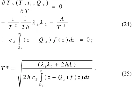
(15)4.SOLUTION PROCEDURE
Using convexity rule, we can obtained three objective variable:
T
*,
t
1*,
Q
s*
. The necessary conditions and the sufficient condition for equation maximizing)
,
,
(
T
t
1Q
sTp
are0
)
,
,
(
;
0
)
,
,
(
;
0
)
,
,
(
1 1 1 1
s s P s P s PQ
Q
t
T
T
t
Q
t
T
T
T
Q
t
T
T
(16) 0 ) , , ( ; 0 ) , , ( ; 0 ) , , ( 2 1 2 2 1 1 2 2 1 2 s s P s P s P Q Q t T T t Q t T T T Q t T T (17)From equation (15), first we can derivative the equation to
Tp
/
Qs
0
, with implies0 ) ( ) ( ) 2 ( ; 0 ) , , ( 1
dz z f T c h p h Q Q t T T s Q k s s P (18)Hence, from equation (18), we can defined the probability of stock out,
,
as
) ( ) 2 ( ) ( T c h p h dz z f k Qs (19)
) 1 (
) 2 1 ( 1
0 ) , , (
1
) ( 1
1
e
b t sb ab p h P T
t Q t T TP
Then
ab
b
e
(b)t1
(20)
Then, we can define t1 using logarithmic rule, as
) (
] / ln[
1
b ab b
t (21)
Third, we can derivative the equation (15) to
Tp
/
T
0
. The optimum value of T can be obtained by solving the equation (15). It is require two substitutions considerably more computational, so we can easily to solve the derivative problem.Let
1
(
P
p
);
and (22)
{
1
1
};
) ( 2 2
1
t
b
b
ab
e
b t (23)The derivative of the latter, according the product-difference rule, after some simplification (see Appendix A3), is
; 0 )
( ) (
2 1 1
0 ) , , (
2 2 1 2
1
dz z f Q z c
T A h
T T
Q t T T
s
Q
s k
s P
(24)
. ) ( ) (
2
) 2 (
* 1 2
dz z f Q z c h
hA T
s
Q
s k
(25)
The optimum value of
T
can be obtained from expression (20). The value of
2T
p/
T
2is always negative to satisfy the sufficient condition for maximizingT
P. The sufficient condition for maximum value of profit is3 2 1 3 2
1 2
2
1
1
)
,
,
(
T
A
h
T
T
Q
t
T
T
P s
(26)
For T > 0, expression (26) always negative.
The optimum value of T can be obtained by solving equation (20). It requires considerably more computation than a non recursive procedure. As a consequence, we suggest slightly modifying the Hadley-Within algorithm as follows:
- Step 1. Start with assumption that t1=T; then find expected TD by solving equation (13). Compute
Dh
A
T
0
2
/
based on Wilson’s model.- Step 2. Compute the probability of stock out,
, by solving equation (19).- Step 3. Compute Qs by assume that demand is normally distributed,
Q
s
T
D
z
T
.- Step 4. Compute the total profit,
T
P0 , by solving equation (14).- Step 5. Go to step 1. To make iteration by increasing
T
, substituteT
i
T
0
T
0 and computeT
Pi by performing Step 2 and Step 3. IfT
Pi >T
P0 , leti i
i
T
T
T
1
then computeT
Pi1. IfT
Pi<T
P0STOP iteration with then go to Step 6.- Step 6. To make iteration by decreasing
T
, substitute 00
T
T
T
i
and computeT
Pi by performing Step 2 and Step 3. IfT
Pi >T
P0 , letT
i1
T
i
T
i then computeT
Pi1. IfT
Pi<T
P0STOP iteration. Hence, the uniqueness of the optimum replenishment policy,T
, can be provided by choosing the bestT
Pi.5. NUMERICAL EXAMPLE AND ANALYSIS
To illustrate the present model, the following examples are considered. The problem to be solved here is that a Grosser sell a single commodity, i.e. garlic, such as in agricultural production, where the output of harvesting is a stochastic environment (i.e. life time and quality).
Example:
Find the optimum replenishment policy, here we have parameters as follows: a=10; b=0.05; A=25,000; h=500; cu=10,000; =0.1; P=10,000; and e=2.71828.
Compute the optimum replenishment policy by the proposed algorithm above:
(1). Compute T0 and TD:
After we calculate based on the proposed algorithm above, after some simplification, then we get:
b+ = 0.15
Ab = 0.5
(b+ab = 0.3
Ln(b+)/ab) = 3.401197
t1={Ln(b+)/ab}/(b+) = 22.67465
Find T0 23
1 = 15,250
2 = 568.86
TD = 798.86
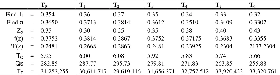
[image:5.595.62.295.397.549.2](2). Find α, Zα, TR, Qs and TP:
Table 2. The optimum replenishment policy
T0 T1 T2 T3 T4 T5 T6
Find Ti = 0.354 0.36 0.37 0.35 0.34 0.33 0.32
Find α = 0.3650 0.3713 0.3814 0.3612 0.3510 0.3409 0.3307
Zα = 0.35 0.30 0.25 0.35 0.38 0.40 0.43
f(z) = 0.3752 0.3814 0.3867 0.3752 0.37175 0.3683 0.3355
(z) = 0.2481 0.2668 0.2863 0.2481 0.23925 0.2304 2137.2304
TC = 5.95 6.00 6.08 5.92 5.83 5.74 5.66
Qs = 282.85 287.77 295.73 279.81 271.83 263.85 255.88
TP = 31,252,255 30,611,717 29,619,116 31,656,271 32,757,512 33,920,423 33,320,761
Computed results and the optimal replenishment policy are shown in Table 2. The optimal value of T and TP are T* = 0.33 and Tp= 33,920,423. This numerical example capture that the grosser should obtained the optimal replenishment policy compare to optimal quantity of commodity to be ordered. Then, based on the optimal replenishment policy, we proposed how many quantity of commodity to be ordered by grosser to get maximum profit.
In our comparison with reference model, it is clear that this model obtains the length of the cycle time then we calculate the quantity of commodity to be ordered by grosser. The reference model derives optimal operating characteristics of the expected cost per unit time. Then, the reference model make the approximate policy by calculate the average deviation to each parameters.
6. CONCLUSION
A stochastic inventory model for deteriorating commodity under stock dependent selling rate and considering selling price was derived by this research. In particular, the optimal replenishment time was derived. Moreover, the numerical examples were shown to evidence the usefulness of the proposed model. By integrating demand depend on selling price between price policy in stochastic market environment, Firms or Grosser can maximize the profit through determine the optimal replenishment time.
In reality, many of the inventory systems dealing with foods items, vegetables, and meats can be tacked by the present model; in which the optimal replenishment time can measured per day, per weeks, etc. due to the commodity’s characteristics. Besides that, the unit in stock can measured per kg, per ton, per stock keeping units (SKU) and etc.
For further research, this model could be extended to other characteristics of deteriorations problems in grosser, in examples with capacitated stored, considering treatment cost to pursuing decay of quality, consider transaction scheme to supplier.
ACKNOWLEDGMENT
The authors are grateful to the anonymous referees for comments and recommendations that improved the paper.
APPENDIX
Appendix A1: The derivation of equation (7)
) ( ) ( )
(
)
(
t t tt
I
bI
a
t
I
, 0tt1
Linier First Order Equation Theorem
) (
)
(
dt A
t y z
vy
e
vdtze
vdtdx dy
-a
z
and
)
(
;
b)
(
Let v
(t)
t
y
t
I
The specific value of the integration can be expressed as,
)
)
(
(
( )) ( )
(
e
A
a
e
dt
I
t bdt
b
Substituting this limit, 0tt1for the equation above and the get the specific value of A, define I(0)=0, then find the specific value of
I
(t), proof of expression (9):} 1 {
)
( ( )(1 )
e
b tt ba t
I
Appendix A2: The proof of equation (18)
Let equation (18),
dz z f Q z T c h
T A Q p h t T a
b t b
ab at
T p h P
t Q t T T
s
Q
s k
s
t b s
P
e
) ( ) (
) (
) 2 ( )] (
} 1
{ [
1 ) 2 1 (
) , , (
1
1 )
( 2 1
1 1
1
We can easily extend to the more function using the role of the derivative of the power-function rule generalized:
)
(t
f'
.
t
y
then
)
c.f(t
y
If
1 11
c
Let us consider a function:
1)} } ) ( { { ) (t f' )} ( } 1 { { ) f(t
(
1 1 1 ) ( ) ( 2 1 1 1 ) ( 2 1 1 e
e
e
t b t b t b b ab a b b b ab a t T a b t b ab at Thus, it is also valid to write:
2 );1 ( 1 } ( ){ 2 1 ( 1 0 ) 1 ( ) 2 1 ( 1 ) , , ( 1 1 ) ( ) ( 1 1 p h P T b ab p h P T b ab p h P T t Q t T T
e
e
t b t b s P The equation can be expressed alternatively as
;
1 ) (ab
b
e
b t
So that a different value of t1 will result in different value of the derivate, such as
)
(
]
/
ln[
1
b
ab
b
t
Appendix A3: the proof of equation (24)
From equation (15), we can easily extend to the more function using the role of the derivative of the product of two functions (product role):
a v p h P T u t T a b t b ab at v p h P T vu ue
b t ' )}; 2 1 ( 1 { ' v and u of derivatif the Find )} ( } 1 { { and ); 2 1 ( 1 u Let ' .v' t y then v(t) . u(t) y(t) If 2 1 1 ) ( 2 1 1
The derivative of the latter, according the product -difference rule, is
0 ) , ,
( 1
T Q t T
TP s
,
Let
1
(
P
p
);
and
{
1
1
};
) ( 2 2 1
t
b
b
ab
e
b t
2 )]1 ( 1 ][ } 1 { [ ) 2 1 ( 1 ' .v' t y 2 1 ) ( 2 1 p h P T aT b t b ab a p h P T vu u
e
b t
Thus, it is also valid to write:
.
)
(
)
(
2
)
2
(
*
1 2dz
z
f
Q
z
c
h
hA
T
s Q s k
REFERENCESAggoun, L., Benkherouf, L. and Tadj, L. (2001). On A Stochastic Inventory Model With Deteriorating Items.
IJMMS, 25:3, 97-203.
Benkherouf, L. and Mahmoud, M.G (1996). On an Inventory Model for Deteriorating Items with Increasing Time-Varying Demand and Shortages. The Journal of the Operational Research Society, Vol. 47: 1, 188-200.
Bose, S., Goswami, A. Chaudhuri, K.S. (1995). An EOQ Model for Deteriorating Items with Linier Time-dependent Demand Rate and Shortages Under Inflation and Time Discounting. Journal of the Operational Research Society, 46, 771-782.
Bounkhel, M., Tadj, L. & Benhadid, Y. (2005). Optimal Control of A Production System With Inventory-Level-Dependent Demand. Applied Mathematics E-Notes, 5, 36-43.
Chung,K-J. and Ting, P-S.(1993). Heuristic for Replenishment of Deteriorating Items with a Linear Trend in Demand. The Journal of the Operational Research Society,
Vol. 44:12,1235-1241.
Research Society, Vol. 50:11, Yield Management, 1176-1182.
Dave, U. (1989). On a Heuristic Inventory-Replenishment Rule for Items with a Linearly Increasing Demand Incorporating Shortages. The Journal of the Operational Research Society, Vol. 40: 9, 827-830.
Dave (1991). Survey of Literature on Continuously Deteriorating Inventory. The Journal of the Operational Research Society, Vol. 42: 8, 725-725.
Ghosh, S.K. & Chaudhuri, K. S. (2004). An Order-Level Inventory Model For A Deteriorating Item With Weibull Distribution Deterioration, Time-Quadratic Demand And Shortages. AMO - Advanced Modeling and Optimization, Vol. 6:1, 21-35.
Giri, B.C., Goswami, A. & Chaudhuri, K. S. (1996). An EOQ Model for Deteriorating Items with Time Varying Demand and Costs. The Journal of the Operational Research Society, Vol. 47:11, 1398-1405.
Goswami, A. and Chaudhuri, K. S. (1991). An EOQ Model for Deteriorating Items with Shortages and a Linear Trend in Demand. The Journal of the Operational Research Society, Vol. 42, No. 12, 1105-1110.
Jamal A. M. M., Sarker, B. R. & Wang, S. (1997). An Ordering Policy for Deteriorating Items with Allowable Shortage and Permissible Delay in Payment. The Journal of the Operational Research Society, Vol. 48: 8, 826-833.
Mehta, N. J., & Shah, N. H. (2003). An inventory model for deteriorating items with exponentially increasing demand and shortages under inflation and time discounting.
Investigação Operacional, 23, 103-111.
Nahmias, S. (1982). Perishable Inventory Theory: A Review. Operation Research, Vol. 30:4, 680-708.
Padmanabhan G. and Vrat P. (1995). EOQ models for perishable items under stock dependent selling rate.
European Journal of Operational Research, 86, 281-292. Raafat, R. (1991). Survey of Literature on Continuously Deteriorating Inventory Models. The Journal of the Operational Research Society, Vol. 42, No. 1, 27-37.
Roy, A. (2008). An inventory model for deteriorating items with price dependent demand and time-varying holding cost. AMO-Advanced Modeling and Optimization,
Vol. 10 :1, 25-37.
Shah, Y. K. and Jha, P. J. (1991). A Single-Period Stochastic Inventory Model under the Influence of Marketing Policies. The Journal of the Operational Research Society, Vol. 42: 2, 173-176.
Demand and Partial Backlogging. The Journal of the Operational Research Society, Vol. 54: 4, 432-436.
Teng, J.-T., Yang, H. -L. & Ouyang, L.-Y. (2003). On an EOQ Model for Deteriorating Items with Time-Varying
AUTHOR BIOGRAPHIES
Wahyudi Sutopo is a lecturer in Department of Industrial Engineering, Faculty of Engineering, University of Sebelas Maret. He is candidate of Ph.D from Bandung Institute of Technology and his dissertation is at supply chain management area. His study is funded by BPPS scholarship program from Directorate General of Higher Education Ministry of National Education, Republic of
Indonesia. His email address is