DOI: 10.12928/TELKOMNIKA.v12i1.1979 135
A New Control Curve Method for Image Deformation
Hong-an Li*1,2, Jie Zhang3, Lei Zhang1, Baosheng Kang1
1 School of Information Science and Technology, Northwest University, Xi’an 710127, China
2
School of Computer Science and Technology, Xi'an University of Science and Technology, Xi'an 710054, China
3
Department of Hematology, Tangdu Hospital, Fourth Military Medical University, Xi’an 710038,China *Corresponding author, e-mail: [email protected]
Abstract
Different from the direct deformation on the image,we propose a deformation method using wavelet filter and control curves. Firstly, the original image is filtered into a high-frequency subimage and a low-frequency subimage by the wavelet, and the low-frequency subimage is deformed use the moving least squares and the control curves.Then, the key points are set to create control curves according to shape information or deformation requirement, and moved to new position to deform the image using moving least squares. At last, the final deformation image can be obtained by adding the deformed low-frequency part to the high-low-frequency part. Experiments show that the proprosed method performs very well to preserve high-frequency detail information and describe the image shape and contour, so can obtain the satisfactory and realistic deformation results.
Keywords: Deformation, Wavelet, subimage, Control Curves
1. Introduction
Image deformation technique has been widely used in our life, such as film and television animation [1], medical image processing [2], etc. The most common image deformation method is to choose some objects to control the deformation, the control objects can be points [3], line segments or polygon meshes [4], so we can do the image deformation by changing the position of the control objects.
Many scholars have proposed various image deformation methods, and they select different control objects to carry out the image deformation. Lee presented the free grid deformation method [5], which can achieve the deformation by the image parameterization using binary cubic interpolation spline, but it need to align the register grid according to image characteristics with the control point spline, and it is Not easy to operate. Beier and Neely improved the free grid deformation technology by using a set of line segments to control the deformation, which is very comfortable to use [4]. Koba used the improved free grid deformation technology in the image surface deformation and obtained a good result [7]. Igarashi put forward a point-based image deformation method [8], it subdivided the input image into triangles, solved the linear equations system with the number of unknown variables equal to the number of all triangle vertexes, which can reduce the distortion degree of the deformed image and keep image deformation as rigid as possible. A common feature of the above methods is to minimize their local scaling and shearing, but these deformation operations are complicated and may be can’t obtain the satisfactory and realistic deformation results.
An novel image deformation method using Moving Least Squares (MLS)Literature [9] was proposed, it established a deformation mapping function of feature points or segments to control different image deformations. The deformation method had a strong sense of reality, and enabled the user to generate a feeling of manipulating real objects. But the method didn't take into account the hierarchical relationships contained in the image, so it is easy to produce bad results with shear, distortion and stretch with wrong proportion, and it is often produce unsatisfactory results in some local areas on the same scaling. So it has some limitations.
2. Wavelet Filter
The wavelet transform is considered to be a new milestone in the development of Fourier transform, it has been regarded as mathematical microscope with excellent "zoom" performance. In the wavelet theory, signal is represented by a weighted sum of a series of basis functions, and the basis functions can be obtained from a wavelet mother function by dilation and translation. Because wavelet function is a short-term shock function with compact support, it has a good local properties in the time domain (spatial) and frequency domain [10]. It is a good tool to extract both detail componets and approximate componets of images because we can do the joint analysis of spatial domain and frequency domain obtained from wavelet transform, and the low frequent part is considered to be the approximate signal and the high frequent part is considered to be the details of signal.
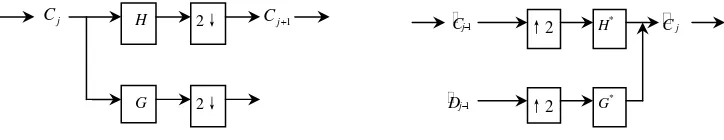
The original image is treated as a signal f t( )and is filtered into different frequency components using Mallat algorithm [11], [12]:
1
. Equation (1) is rewritten into a matrix form:
1 , 1 1,2, ,
j j j j
C HC D GC j J (2)
Where, J is the wavelet decomposition level. Equation (2) is the Mallat pyramidal decomposition algorithm, whose process is shown in Figure 1. Where, 2 is the value of only even location.
Figure 1. Decomposition of Mallat Figure 2. Reconstruction of Mallat
After f t( ) is decomposed using the Mallat algorithm, the signal is distinguished from noise based on the experiential information, and then f t( ) is filtered to generate a new sequence Cj and Dj. The Mallat reconfiguration algorithm is : Where, 2 is the liter sample, it means that the number of samples is 2 times than the original.
When the signal is reconstructed, the part which is relative to the high frequency detail signal is deleted, then the filtered signal is obtained:
Equation (4) is a smooth signal expression after f t( ) is filtered. It is equivalent to using a smooth curve to fit it [12].
We can use the high and low frequency of image to measure the changing intensity of different locations. In proposed method we filter out the high frequency part of image by wavelet
obtain the final result of image deformation by adding the deformed low frequency part to the high frequency part of the original image. Figure 3 shows the algorithm process.
Figure 3. The process of image deformation based on wavelet filter using control curves and MLS
3. Image Deformation using Moving Least Squares
The whole Moving Least Squares deformation algorithm process is to find the mapping function f , where the image before deformation is regarded as an independent variable, and the deformed image is regarded as target variable. Figure 4 shows an example of image deformation. Figure 4(a) is the original image and Figure 4(b) is the corresponding deformed image, which is obtained by employing deformation function f .
(a) Original (b) Deformed
Figure 4. Image deformation
According to moving least squares theoretical model [8], assuming that S is the feature points set of original image and D is the feature points set of deformed image, there is a deformation function f which can make the value of expression (5) minimum.
2| |
i
i i
w f s d
(5)2
1 | |
i i
w
s v
(6)
Where, wi is weight and its value varies according to the position of v in the image, and v stops moving when corresponding value of expression (5) is minimum, so the method is called MLS [9]. When v is equal to si, weight value wi is infinite, so define f s
i di; Whenfeature point si does not vary, define f s
i si di.
f x xM T (7)
Where, M represents linear transformation, and T represents translation transformation.
/ /
i i i i i i
i i i i
T w d w w s w M
(8)
i i / i i i / iSo the expression (9) can be rewritten into:
2
The process of the MLS image deformation algorithm is as follows:
Step 1. Select feature points set S{ , ,s s1 2,sn} in the original image Figure 5(a).
Step 2. Determine the positions of s in the deformed image Figure 5(b), which can be denoted as a new feature points set D{ ,d d1 2,,dn}.
Step 3. Determine the mapping function f according to di f s( )i .
We can obtain the deformed image by applying mapping f to the remaining points of original image. Linear transformation M can be affine transformation, similarity transformation and rigid transformation. Also we can use forward mapping or reverse mapping to generate a new image. Because the forward mapping is prone to produce voids and overlapping phenomena, so we use the reverse mapping in this paper. Figure 5 shows the MLS image deformation effects [9].
a) Original (b) Affine (c) Similarity (d) Rigid
Figure 5. Image deformation based on MLS
Where, Figure 5(a) is the original image, Figure 5(b) is an affine deformed image, Figure 5(c) is a similarity deformed image, and Figure 5(d) is a rigid deformed image. There is serious wrong shear phenomenon and uneven scaling transformation in Figure 5(b). The effect of Figure 5(c) is better than Figure 5(b), but there is proportional distortion in the right part of image in Figure 5(c). Figure 5(d) is better, the deformation result is close to the real objects. Therefore, this paper adopts the rigid deformation.
(a) Original image (b) Deformed image (c) Deformed image
Figure 6. Image rigid deformation
4. Control Curves
We use cubic spline curve fitting method to generate the control curves, so as to better control the path of control curves [13], [14]. The cubic spline curve piecewise fits the control points, so the curve can pass the control points accurately and has second order continuity on the connection point. Control points can be got by clicking the mouse. In order to generate a curve which includes n segments we need to use n1 orderly control points
( 0, 1, 2, , ) j
a j n . Each segment is generated using cubic spline curve, and the cubic spline
curve is generated using the free endpoint conditions. Assume that s ii( 0, 1, 2,, )n is the ith control curve before deformation, the d ti( ) is the corresponding ith curve after the deformation, its corresponding n1 ordered control points are b jj( 0, 1, 2,, )n , and t(0, 1). According to the expression (1) we can obtain:
1 2
. Solving the above equation and
getting the minimum value of expression (12) we can obtain:
* *
Expression (12) can be rewritten into:
1 coordinates, and the value can be calculated by the free endpoints. Similarly, bi1 and biare respectively the start and end coordinates of the ith curve after image deformation, bi1 and bi are respectively the first derivative values of start and end coordinates. According to equation (16), the expression of cubic spline curve can be rewritten into:
3 2
We can generate cubic spline curve on the free endpoints according to the expression of (17) and (18), so the control curve set S and D are generated. Match the points in S with the points in D, use them as control points, and deform the image based on the control points set method.
5. Experiments
5.1. Feature points extraction
In our experiment, we validate the proposed method on face images. According to the deformation requirement of face image, we define 68 face feature points which refer to the definitions of face feature point parameters in MPEG-4 [15]. The face feature points mainly locate at outside contour of face, eyebrows, nose and mouth, and relatively dense feature points are set to the facial features region, which is the main part of deformation and action [16]. Facial feature points include two kinds, one is the organ description feature points and the other is the basic feature points which are also called contour feature points. Basic feature points describe the whole facial external characteristic, which is denoted as hollow dots in Figure 7, they divide a whole face according to facial shape features, determine the characteristics of the face and the major organs, which is the important reference standard for establishing face deformation feature points.
Figure 7. The MPEG-4 definition of the human face features [15]
5.2. The algorithm of image deformation based on wavelet filter using control curves Input the original image which need to be deformed, and carry out the following steps: Step1. Set key points, create a control curve set S, represent the contour or shape of image. Step2. Move the points, change the position and direction of the spline curves, generate a
deformed control curve set D.
Step3. Make one-to-one correspondence between the control points of S and D by calculation, generate the control points.
Step4. Filter the original image into a high-requency part and a low-frequency part. Step5. Deform the low-frequency part using the control points method.
Step6. Add the deformed low-frequency part to the high-frequency part of the original image, obtain the final deformation image.
5.3. Experiment results
We use the Matlab 2011b in the experiments, and Figure 8 shows the deformation results.
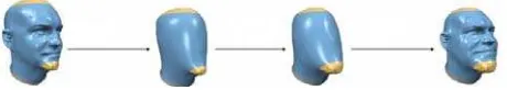
(a) Original (b) MLS (c) MLS (d) our method
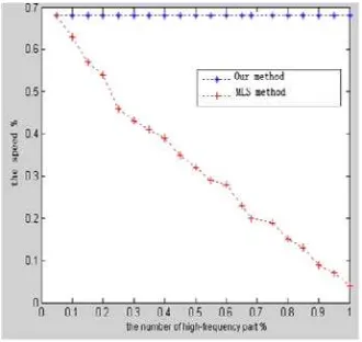
Figure 8. Image deformation results Figure 9. The compare of speed
The Figure 8(a) is an original image, the Figure 8(b) and the Figure 8(c) are the deformed images using MLS, and the Figure 8(d) is the deformed image using our method. As can be seen from the deformation effect, our method can keep enough image details, and there is no local distortion and tension phenomenon which can be seen in the Figure 8(b) and the Figure 8(c), in addition to this, our deformation is more smooth and realistic. Owing to the high-frequency part of the image has been filtered out,The differences between points in the low-frequency part have been significantly reduced. Besides, we only deal with the edge and contour of the image during the deformation process, so can retain the high-frequency information completely. Because using the control curve set to describe the shape topology relations or contour information and deforming the different parts of the contour and edge in different scales, the different parts of the contour and edge can keep their shapes, and the final deformation effect will be more natural and smooth, it is the reason that our method can greatly improve the fitting effect.What's more, our method can greatly increase the deformation speed because it will reduce the number of feature points (the Figure 9).
6. Conclusion
calculation precision are improved; Because using different scales to deform the different parts of the contour and edge of the image, the shape and contour of the image are well described; Because reserving the high-frequency information of the image completely, the detail is clear and the deformation is smooth.
Currently, due to the rapid development of computer hardware, 3D model has become another major treatment target in the field of visualization techniques [17]. In the future work, we intend to apply our method in the deformation of the 3D model,so that can otain more smooth and natural deformation effects.
Acknowledgment
This research is supported by the National Natural Science Foundation of China (Granted No. 61272286).
References
[1] Smythe, D.B. A two-pass mesh warping algorithm for object transformation and image interpolation. Tech. Rep. 1030, ILM Computer Graphics Department. 1990.
[2] Bookstein, F. L. Thin-plate splices and the decomposition of deformations. IEEE Transactions on Pattern Analysis and Machine Intelligence. 1989; 11(6): 567–585.
[3] McCracken, R and Joy, K. I. Free form deformations with lattices of arbitrary topology. In Proceedings of ACM SIGGRAPH 1996, ACM Press. 1996: 181–188.
[4] Beier, T. and Neely, S. Feature based image metamorphosis. Proceedings of the 19th annual conference on Computer graphics and interactive techniques, ACM Press, NY, USA. 1992: 35–42. [5] Lee, S., Chwa, K. and Shin, S. Image metamorphosis using snakes and free-form deformations. In
SIGGRAPH 1995: Proceedings of the 22nd annual conference on Computer graphics and interactive techniques, ACM Press, New York, USA. 1995: 439–448.
[6] Warren, J., Eechele, G., and Thaller, C., etc. A geometric database for gene expression data. Proceedings of the 2003 ACM SIGGRAPH symposium on Geometry processing. 2003: 166–176. [7] Koba yashi, K. and Otsubo, K. Free form deformation by using triangular mesh. Proceedings of the
eighth ACM symposium on Solid modeling and applications, ACM Press. 2003: 226–234.
[8] Igarashi, T., Moscovich, T., and Hughes, J. F. As rigid as possible shape manipulation. ACM Trans. Graph. 2005; 24(3): 1134–1141.
[9] Schaefer, S.,McPhail T. and Warren J. Image deformation using moving least squares. ACM Transactions on Graphics. 2006; 25(3): 533–540.
[10] FAN Chunnian, WANG Shuiping, ZHANG Fuyan. Wavelet-based illumination normalization algorithm
for face recognition. Computer Engineering and Applications. 2010; 46(6): 174–177.
[11] Zhang Xiangwei, Luo Shaoming, Zhong Tongzi. Wavelet Analysis in Testing Signal. Applied Mathematics and Mechanics. 1998; 19(3): 203–207.
[12] Ma Pan, Meng Lingkui, Wen Hongyan. Kalman Filtering Model of Dynamic Deformation Based on
Wavelet Analysis. Geomatics and Information Science of Wuhan University. 2004; 29(4): 349–353.
[13] Hua Shungang, Liu Ting. Study on image deformation based on moving least squares. Journal of Computer Applications. 2009; 29(1): 71–73.
[14] Hua Shungang, Li Xiaoxiao, Li Shaoshuai. Image Deformation Using Control Curves and Moving
Least Squares. Journal of Chinese Computer Systems. 2010; 31(11): 2251–2254.
[15] ISO/IEC JTC1/SC29/WG11 Document N3908, MPEG4 Video Verification Model version 18.0. 2001. [16] Qiang Zhang, Yuan Xu, Changjun Zhou. A Novel DWT-Based Watermarking for Image with the SIFT.
TELKOMNIKA. 2013; 11(1): 191–198.
[17] Xiuping Ping. The Reserch of Granular Computing Applied in Image Mosaic. TELKOMNIKA. 2013; 11(3): 537–546.
![Figure 7. The MPEG-4 definition of the human face features [15]](https://thumb-ap.123doks.com/thumbv2/123dok/236288.502123/6.595.102.498.559.668/figure-mpeg-definition-human-face-features.webp)