On determining spectral parameters, tracking jitter, and GPS
positioning improvement by scintillation mitigation
Hal J. Strangeways,
1Yih
‐
Hwa Ho,
2,3Marcio H. O. Aquino,
4Zeynep G. Elmas,
4H. A. Marques,
5J. F. Galera Monico,
5and H. A. Silva
5Received 29 November 2010; revised 10 April 2011; accepted 4 May 2011; published 4 August 2011.
[1]
A method of determining spectral parameters
p
(slope of the phase PSD) and
T
(phase PSD at 1 Hz) and hence tracking error variance in a GPS receiver PLL from
just amplitude and phase scintillation indices and an estimated value of the Fresnel
frequency has been previously presented. Here this method is validated using 50 Hz
GPS phase and amplitude data from high latitude receivers in northern Norway and
Svalbard. This has been done both using (1) a Fresnel frequency estimated using
the amplitude PSD (in order to check the accuracy of the method) and (2) a constant
assumed value of Fresnel frequency for the data set, convenient for the situation when
contemporaneous phase PSDs are not available. Both of the spectral parameters
(
p
,
T
) calculated using this method are in quite good agreement with those obtained
by direct measurements of the phase spectrum as are tracking jitter variances determined
for GPS receiver PLLs using these values. For the Svalbard data set, a significant
difference in the scintillation level observed on the paths from different satellites
received simultaneously was noted. Then, it is shown that the accuracy of relative GPS
positioning can be improved by use of the tracking jitter variance in weighting the
measurements from each satellite used in the positioning estimation. This has significant
advantages for scintillation mitigation, particularly since the method can be accomplished
utilizing only time domain measurements thus obviating the need for the phase PSDs
in order to extract the spectral parameters required for tracking jitter determination.
Citation: Strangeways, H. J., Y.-H. Ho, M. H. O. Aquino, Z. G. Elmas, H. A. Marques, J. F. G. Monico, and H. A. Silva (2011), On determining spectral parameters, tracking jitter, and GPS positioning improvement by scintillation mitigation,Radio Sci.,46, RS0D15, doi:10.1029/2010RS004575.
1.
Introduction
[2] It is well known that GNSS satellite systems operating in L band are subject to ionospheric amplitude and phase scintillation effects and, in the equatorial region, (±20° geomagnetic latitude), these are generally most prominent for a few hours after local sunset. In the high latitude (polar and auroral) regions, phase scintillation is more dominant than amplitude scintillation and can occur at any time during the day especially during geomagnetic storms. In midlati-tude regions, both amplimidlati-tude and phase scintillation are negligible. Amplitude scintillation is more dominant at low
latitudes and phase scintillation at high latitudes. The scin-tillation arises from ionospheric irregularities which can be embedded in mesoscale structures such as polar patches or low latitude plasma bubbles. Such scintillation has an adverse effect on GPS range estimation and on positioning by introducing tracking jitter variance in receiver PLLs, which can lead to cycle slips and, for sufficiently strong scintillation conditions, even loss of carrier phase lock. It is therefore desirable to be able to mitigate the scintillation effect. This can be attempted via receiver hardware mod-ifications (e.g., to make the phase tracking more robust) or by software means. The latter can involve either leaving out the satellites in the positioning calculation whose paths to the receiver have been severely affected by scintillation [Beniguel et al., 2004] or weighting all the satellites in the positioning calculation inversely according to the scintilla-tion present on the respective satellite to receiver paths. This can be done by utilizing the estimated tracking error var-iances in the receiver PLL for each satellite receiver path to weight the respective ranges in the positioning calculation [Aquino et al., 2009]. These variances can be determined for GPS receivers from the formulae given byConker et al. [2003] if the spectral parameters p (slope of the phase
1
School of Electrical, Electronic and Computer Engineering, Newcastle University, Newcastle, UK.
2
School of Electronic and Electrical Engineering, University of Leeds, Leeds, UK.
3
School of Electronics and Computer Engineering, Universiti Teknikal Malaysia Melaka, Melaka, Malaysia.
4
Institute of Engineering Surveying and Space Geodesy, University of Nottingham, Nottingham, UK.
5Department of Cartography, Sao Paulo State University, Presidente
Prudente, Brazil.
spectrum plotted on log‐log axes) and T (phase power spectral density at 1Hz) are known. We will follow a similar procedure here but instead of determining the spectral parameterspandTfrom the phase spectrum (which requires high rate raw data of carrier phase and continuous FFTs to be performed on this data for all the satellites) or from estimatingpjust based on the prevalent conditions which is rather difficult [Aquino et al., 2007], we will instead obtain them from the scintillation indices using the method of Strangeways[2009, hereinafter S09].
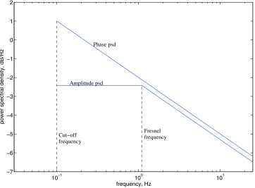
[3] In the S09 method, the phase parameters are deter-mined directly from the phase and amplitude scintillation indices making use of approximate models of the amplitude and phase spectra and an approximate value for the Fresnel frequency for the path. The Fresnel frequency is an impor-tant feature of the amplitude PSD and is given by the velocity of the scintillation‐inducing irregularities perpen-dicular to the satellite to receiver path divided by the Fresnel scale. The phase and amplitude spectra are modeled as shown in Figure 1 (except that the sloping parts of the spectra are assumed to coincide whereas they are shown a little separated in Figure 1 for clarity). Rino’s [1979] rep-resentation of the phase scintillation PSD is given by:
S¼
where f0 is the outer scale, p is the spectral slope of the phase PSD and Tis its spectral strength at 1 Hz. If ff0 then we can writeS=Tf−p
. Then the variance of the phase of the detrended GPS phase data (equivalent to the scintil-lation indexs8
2
) is equal to twice the area under the curve S (f) (also determined from the PDF of the detrended phase
data) and thus corresponding to the same range of fading frequency between a lower cutoff frequency fc(generally set by the detrending filter) and an upper cutoff frequency fu (generally given by half the sampling frequency). A similar relationship will exist between the (normalized) amplitude scintillation index sc and the area under the curve of
the PSD for amplitude. Both these relations follow from Parseval’s theorem for discrete signals. Then the difference in the squares of the scintillation indices must be equal to twice the difference in these areas yielding [Strangeways, 2009]:
2
wheresc, the (normalized) amplitude scintillation index, is
equivalent to S2 andS4≈2sc, (providing that, for the
dis-tribution of amplitude, the variation from the mean is much less than the mean; e.g., seeYakovlev[2002] who takes S2 = 0.52S4).fcis the lower cutoff of the detrended data generally
given by high‐pass filter cutoff used for detrending it,fuis
upper cutoff frequency (generally given by half the sampling frequency) andr= 1−p. Then, utilizing a known or estimated
value of the Fresnel frequency (fF), we can find the value of the slope of the phase spectrum p that will result in given values ofs8sandscby finding the zero of the function:
2
tillation indices determined from the detrended data. The Figure 1. Models of the phase and amplitude spectra.
STRANGEWAYS ET AL.: S09 METHOD AND SCINTILLATION MITIGATION RS0D15
precision of the value of the upper cutoff in equation (3) is not so important as long as it is above the Fresnel frequency. However, the value of the lower cutoff can have a signifi-cant effect on the value of s8 since there is a power law
increase is the PSD (resulting from scintillation) with decreasing frequency. Thus it is important that equation (3) is solved for the correct value, which should in any case be known, as otherwise the value of s8 itself is of limited
usefulness. Equation (3) is solved in MATLAB by an algorithm that uses a combination of bisection, secant, and inverse quadratic interpolation methods. This equation can be modified to include the effect of filter roll‐off, an irreg-ularity outer scale or other factors that modify the fading spectrum as explained in section 7 of Strangeways[2009]. Whenphas been found,Tcan then be determined from the relation between p,Tand s8
2
given above.
[5] Since no experimental verification of the method was given by Strangeways [2009], before utilizing it to obtain tracking jitter values to use in weighting individual satellite links, or for other purposes, we will first establish the reli-ability of the method from experimental data. This will be accomplished using 50 Hz amplitude and phase data together with the corresponding scintillation indices (S4 and s8)
from high latitude receiving stations at Tromso (69.67°N, 18.97°E) and Longyearbyen (78.169°N, 15.992°E). Once the spectral parameters are known then the tracking jitter can be determined using the formulae given byConker et al. [2003] who introduced the model of tracking error variance at the output of the L1 carrier PLL as:
2 noise and the oscillator noise components of the tracking error variance respectively. Amplitude scintillation is modeled as:
2
where Bn is the L1 third‐order PLL one‐sided bandwidth (∼10 Hz); (c/n0)L1−C/Ais the SNR andhis the predetection
integration time (0.02s for GPS and 0.002s for WAAS). The formula is valid for S4(L1) < 0.707 and so does not apply to the strongest amplitude scintillation conditions.
[6] The representation of phase scintillation ofRino[1979] was used to calculate the phase error at the input of the PLL by:
2 ¼2
Z ∞
Spð Þf d f; ð6Þ
wheretis a system parameter relating to the phase stability
time of the receiver. Then the phase scintillation component of the tracking error variance at the output of PLL is given by [Conker et al., 2003]:
where kis the order of the PLL,fnis the loop natural fre-quency. Thus the formula gives the tracking jitter in terms of
the characteristics of the phase lock loop, the phase stability of he receiver and its oscillator phase noise, the CNR, the parametersp andT of the phase spectrum of the detrended signal and the amplitude scintillation index S4. For the calculations of tracking jitter presented belowkwas taken as 3,h as 0.02, fnas 1.91 Hz, Bnas 10 Hz, sOSCas 0.1 rad.
and (c/n0)L1−C/Awas obtained from the receiver each minute.
2.
Experimental Validation of the Method
of Determining Spectral Parameters
From Scintillation Indices
[7] The S09 method has been investigated using both high latitude 50Hz GPS amplitude and phase data. This has been done both using (1) using fixed values of the Fresnel frequency estimated for the conditions and (2) a Fresnel frequency determined from the amplitude spectrum. The latter is performed just to test the accuracy of the method since, if spectra are available to determine this frequency, p and T could be determined from it and there would be no need for the method. In order to check its accuracy values ofpandT, determined by the method, are compared with those determined directly from the phase spectrum.
2.1. Tromso Data
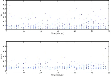
[8] The first example is for 50 Hz GPS data recorded at Tromso on 23 April 2004 from 22:00 to 23:00 UT for SV14 and for GPS frequency L1. The values of S4 (corrected for ambient noise) and Phi60 (s8determined over a 60s period)
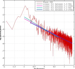
Figure 3. Straight line fitting to the phase PSD to determinep. Figure 2. Carrier to noise ratio, S4 and Phi60 for the 60 min data set.
STRANGEWAYS ET AL.: S09 METHOD AND SCINTILLATION MITIGATION RS0D15
0.15 to 2.5 Hz for high latitudes [Forte and Radicella, 2002]. This has the advantage of removing the problem due to noise at higher fading frequencies so that determined values of p can be found to be larger than those measured from the phase spectrum, which have been underestimated due to this noise effect. This also means that one cannot expectp values obtained by these two methods to agree to a high degree of precision. It might be suggested that the equivalent area under the phase PSD curve has been underestimated on the basis of the phase spectrum model
(as shown in Figure 1) due to the detrending filter reducing the phase PSD just above the lower cutoff. However, careful consideration shows that this is not the case because of added“area”due to the fact that the PSD does not cutoff abruptly at frequencies below the lower cutoff.
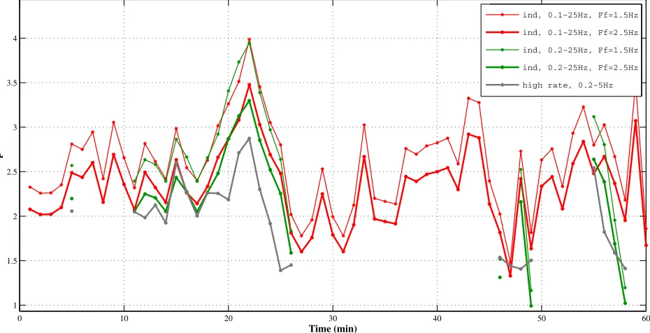
[9] Figure 5 shows the values of p determined from the phase spectrum for the above mentioned data set for the frequency range of 0.2–5 Hz. We expect the values of p obtained for the frequency range of 0.2–5 Hz (“high rate” time series in Figure 5) to be the most accurate as in this Figure 4. Determination of spectral slope, p, over four different frequency ranges.
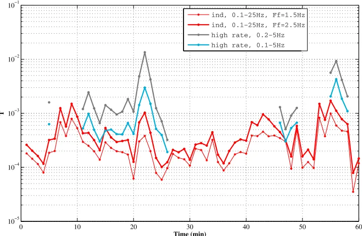
case the above mentioned error sources (such as the noise contribution at the higher frequency part of the spectrum) are removed; thus better representation of the true scintil-lation effect is attained. These are then plotted in Figure 5 together with values from the S09 method (“ind”results in Figure 5) assuming lower cutoffs of both 0.1 and 0.2 Hz and Fresnel frequencies of both 1.5 and 2.5 Hz. Of course for the determination for the 0.2 Hz cutoff, the phase scin-tillation index was recalculated for the high rate phase data detrended with an 0.2 Hz cutoff. It can be seen that there is reasonable agreement especially in the trends between thep values determined for the two methods particularly for the higher value of the Fresnel frequency (2.5 Hz). It can also be seen that thepvalue obtained from the S09 method is not a strong function of the Fresnel frequency assumed. Values of T determined from both methods are shown in Figure 6, where “ind” refers to the results obtained from the S09 method based on the scintillation indices and comparison is made between these outputs and those obtained from processing the high rate data. More accurate estimates may be expected when the high rate data is processed, however the computational effort required is greatly decreased with the S09 method, which gives results that show good agreement overall with those obtained from the high rate data.
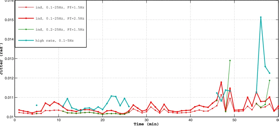
[10] The tracking jitter variances calculated using the determined values of p and T for both methods (“ind”for S09 method and using the high rate data) are shown in Figure 7, where it can be seen that there is approximate agreement except at around minute 57. Whereas the jitter calculated from the high rate data represents more sensitivity to the scintillation effects (dominant around minutes 22 and 55 as understood from Figure 2), those calculated from the scintillation indices are continuous in time since they are not affected by the gaps in the high rate data as severely as the former.
2.2. Longyearbyen Data
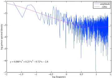
[11] In the next example the Fresnel frequency is deter-mined from the amplitude spectrum using the amplitude PSD. This is in order to check the accuracy of the S09 method for the actual corresponding Fresnel frequency although, in the real application of the method, this would not be done as p could also be found from the amplitude spectrum if this were available. The GPS data is from a receiver at Longyearbyen (78.169°N, 15.992°E), for a time period of 19:00–20:00 UT on 7 May 2008 and for PRN 9 [Romano et al., 2008]. The data was chosen for a time of high scintillation with S4 values for L1 up to 0.6 and s values even exceeding 1. An example of the phase and amplitude spectra is shown in Figure 8. When considering these spectra in the context of the proposed method, it needs to be taken into account that the area between the spectra is proportionally larger and shaped differently from that area between the amplitude and phase spectrums seen in Figure 8 or an“ideal”triangular area as shown in Figure 1. This is because, in both these cases, the spectra are shown on axes of both log amplitude and log frequency, whereas the areas only appear correctly (and in the S09 method are so calculated) when both scales are linear. It is difficult to visually determine the Fresnel frequency directly from the amplitude spectrum as there are insufficient points at lower frequency due to the short time duration of 1 min and finite (50 Hz) sampling rate. Also, the spectrum is too variable to precisely determine the frequency at which a distinct change in slope occurs. The Fresnel frequency was obtained by first making a cubic fit to the amplitude spectrum (see equation (3) ofVan Dierendonck[1999]) over the frequency range 0.2– 5 Hz where most of the scintillation power normally exits for GPS L band signals received at high latitudes. The value of Fresnel frequency was calculated by solving for the zero of the second derivative of the cubic function with Figure 6. T values determined from S09 method and from phase spectrum measurement.
STRANGEWAYS ET AL.: S09 METHOD AND SCINTILLATION MITIGATION RS0D15
respect to frequency, corresponding to the point of inflec-tion where the curvature of the amplitude PSD changes direction. This was regarded as preferable to finding the local maximum (zero of the first derivative) as this could be below the Fresnel frequency. Since the amplitude PSD was obtained for every 1 min (corresponding to 3000 data points) via FFT, values of fF could be computed every
minute from the data. The Fresnel frequency was only determined to investigate whether the method could give an accurate value for p and T if a correct value of Fresnel
frequency was employed. An example of a fitting and the resultant equation is given in Figure 9, where the point of inflection in the curve is indicated. Figure 10 shows the variation of the determined Fresnel frequency over the hour data interval. Sometimes a too high Fresnel frequency is obtained but it was found that fitting the cubic over a wider frequency range could ameliorate this problem.
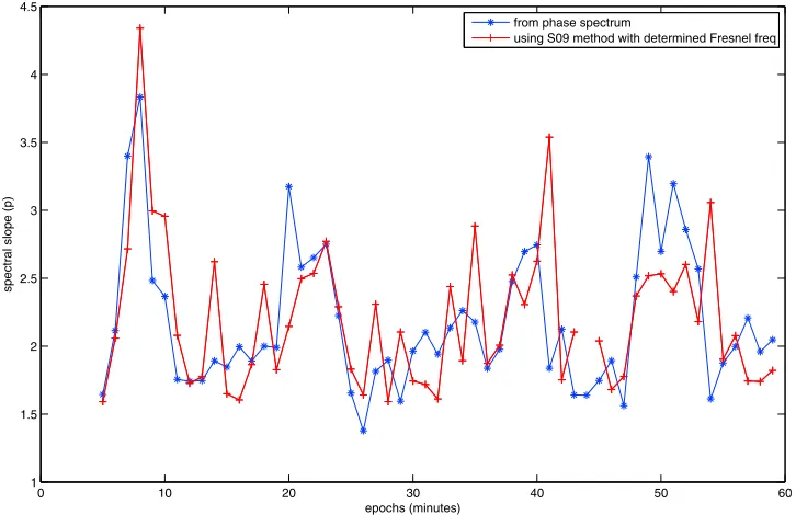
[12] Determined values of p using the S09 method are shown in Figure 11. Values ofpdetermined from the phase spectrum using a straight line fit to the slope of the phase
Figure 8. Example of phase and amplitude spectra from the Longyearbyen (78.169°N, 15.992°E) data set for the period 19:00–20:00 UT on 7 May 2008 and for PRN 9.
PSD are shown for comparison. It can be seen that there is quite good agreement between thepvalues calculated using the two methods. Thepvalues obtained when a fixed value of 3 Hz for the Fresnel frequency was employed are also shown. It can be seen that using the constant value of 3 Hz for the Fresnel frequency does not introduce a significant difference to the determined values ofp. This shows that an
estimated value offF is sufficient. Thepvalues determined from the phase spectrum were obtained by programmed fitting over the total range of 0.1–25 Hz. It can be seen that the profile of the variation of p with time is quite similar for both methods but the values obtained from the phase spectrum are consistently lower. If thepvalues are determined instead from the phase spectrum over the range 0.2–5 Hz (i.e., Figure 9. Example of Fresnel frequency determination by cubic fitting to the amplitude spectrum from
the data set of PRN9 received at Longyearbyen at 19:00–20:00 UT on 7 May 2008.
Figure 10. Fresnel frequency determined from amplitude PSD.
STRANGEWAYS ET AL.: S09 METHOD AND SCINTILLATION MITIGATION RS0D15
excluding the noise contribution from the high frequency part of the spectrum and the lowest frequency portion 0.1–0.2 Hz) they are significantly higher, as shown by the blue curve in Figure 12 (compare with the blue curve in Figure 11), where comparison is again made with the values determined from the S09 method using the determined Fresnel frequency and quite good agreement is found. The values of the phase power spectral density at 1 Hz,T, also show quite good agreement both in trend and magnitude between the two methods, as
shown in Figure 13. A comparison was made between the tracking jitter variance calculated (1) using direct measure-ment of spectral parameterpfrom phase spectra and (2) using a Fresnel frequency determined from the cubic fit to the amplitude spectra. This is shown in Figure 14, where there is approximate agreement between the averages of each time series but less correlation than was seen for the spectral parameterspandT. This is not surprising as the tracking jitter Figure 11. Spectral slope,pfound from the phase PSD (between 0.1 and 25 Hz) and using S09 method
with Fresnel frequency determined from the amplitude spectrum and with a fixed Fresnel frequency of 3 Hz.
variance depends on both parameterspand T and so is sen-sitive to any difference in both between the two methods.
3.
Mitigation of the Scintillation in Positioning
[13] For this data set, it is found that there was a signifi-cant difference in the scintillation level observed on the paths from different satellites received simultaneously at the receiver location. SinceAquino et al.[2009] found that the positional accuracy can be improved by use of the tracking jitter variance to weight the measurements from
each satellite in the positioning calculation, this method was tried on this data set in order to quantitatively determine the improvement in positional accuracy that can be achieved. This was done by using weights derived from the deter-mined tracking jitter variances for each satellite using the S09 method of finding the spectral parameters and the Conker et al. [2003] formulae. This has significant advantages for scintillation mitigation since this process can be accomplished utilizing only time domain measurements, thus obviating the need for continual determination of phase PSDs via FFTs.
Figure 13. Comparison ofT(spectral strength at 1 Hz) determined by the two methods.
Figure 14. Comparison of tracking jitter variance usingpand Tvalues from the two methods.
STRANGEWAYS ET AL.: S09 METHOD AND SCINTILLATION MITIGATION RS0D15
[14] Figure 15 shows the large variation of scintillation, as measured by the S4 index, that can occur between simul-taneous paths from different satellites to the same receiver. This example is for a receiver located in Longyearbyen during the period of 19:00–20:00 UT on 7 May 2008. It illustrates the advantage that weighting the measurements on each satellite‐receiver path according to the scintillation occurring on them could bring to better estimating the
position of the receiver. Normally the observations to all satellites in GPS data processing are assumed to be inde-pendent and of the same quality (same variance, i.e., same weight) disregarding the fact that each satellite to receiver path could be affected differently by the propagation envi-ronment. In reality, of course, they can be affected differ-ently by various factors such as elevation, orientation to the geomagnetic field direction, troposphere effects as well as Figure 15. Scintillation level S4 for four different simultaneous satellite paths to the receiver located in
Longyearbyen during the period of 19:00–20:00 UT on 7 May 2008.
ionospheric scintillation. The latter can clearly affect each satellite to Earth path differently, particularly when con-sidering the fact that scintillation‐inducing electron density irregularities can occur in patches in the ionosphere.
[15] The approach described in detail byAquino et al. [2009] was then used to mitigate the scintillation effects on different satellite‐receiver paths by redefining the stochastic model of the Least Squares adjustment used in estimating the position. This is achieved by computing the GPS observables variances based on the jitter variances. Each satellite to receiver path is assigned its own individual variance and these are propagated according with the algorithm used in the least squares process. In this case a baseline between stations Longyearbyen (LYB0) and Ny Alesund (NYA1) was pro-cessed in relative mode using a double difference algorithm.
This was done using the program GPSeq [Monico et al., 2006], which incorporates the above method. This baseline is∼125 km and data was processed for the period of 19:00–
20:00 UT on 7 May 2008. The S4 and Phi60 indices for this period from all GPS satellites in view at an elevation above 10° are shown in Figure 16. GPSeq allows GPS recursive processing using pseudoranges and carrier phase double differences simultaneously. GPSeq can process the data either in a “nonmitigated” mode (when all satellites observations are assumed to be independent and of the same variance) or in a “mitigated”mode, when the above method is applied. The standard deviations adopted for the code and carrier phase observables in the nonmitigated mode are shown in Table 1. From the time series shown in Figure 17 for the height error and in Figure 18 for the 3‐D Figure 17. Height error for mitigated and nonmitigated solutions.
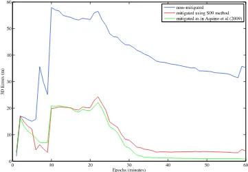
Figure 18. Three‐dimensional position error for mitigated and nonmitigated solutions.
STRANGEWAYS ET AL.: S09 METHOD AND SCINTILLATION MITIGATION RS0D15
positioning error, it can be seen that the positioning accuracy has been improved quite significantly when the above described scintillation mitigation using the S09 method is applied (red curve). There is more than 50% improvement for the average height errors during this 1 h data period and more than 70% improvement in the 3‐D positioning error (Table 2). Also shown in Figures 17 and 18 is the mitigated solution (green line) when the method ofAquino et al.[2009] is used instead which differs in that the spectral parametersp andTused in the determination of tracking jitter (employed to determine the respective weights of the paths in the positioning determination) are found from the phase spec-trum rather than the scintillation indices. It can be seen that there is little difference between the results between the two mitigation methods and both show a significant reduction in positional error compared with the unmitigated solution.
4.
Conclusions
[16] Determination of the tracking jitter using only scin-tillation indices and an estimated Fresnel frequency using the S09 method has been investigated using real data con-taining notable scintillation effects. The results show that a fairly good agreement between p and T values calculated from the S09 method and directly from the phase spectrum can be obtained when care is taken over the frequency range for the linear fit on the phase PSD for the latter. The resultant values from the S09 method are not strongly dependent on the value of the Fresnel frequency if realistic values are used. Furthermore it is found that by utilizing the formulae ofConker et al.[2003] the S09 method can be also employed to reliably estimate the tracking jitter when only the scintillation indices are available or to greatly reduce the computational effort even when they are. Using this method associated with the strategy of Aquino et al. [2009] to determine weights for each signal path depending on the tracking jitter variances in the receiver PLLs, it is found that the accuracy for a data set corresponding to strong scintil-lation conditions was improved by 52% in the vertical component and 71% for the 3‐D positioning error. When the method of finding the tracking jitter to determine the weights, as employed by Aquino et al.[2009], was applied to the same data, similar results were achieved as can be seen from the comparison in Figures 17 and 18 but using the S09 method obviates the need for applying FFTs to deter-mine spectra and then finding p and Tand hence tracking jitter from them. This process would need to be performed every minute for every satellite to receiver path used in the positioning determination.
[17] Then from the comparison in section 2 and the mit-igation results in section 3 it would appear that the tracking jitter values calculated from the spectral parameters esti-mated by the S09 method represent a reliable measure for use in evaluating the GNSS receiver performance during scintillation.
[18] It should be noted that the results presented in this paper are the outcome of an analysis carried out based only on a limited data set that was available to the authors. Clearly, follow‐on research should be carried out involving the analysis of longer and more varied data sets in order to fully validate the method. This will be the subject of future work, which should be enabled by the acquisition of a large amount of new data to be collected in the next 3 years both for high and equatorial latitude conditions in the framework of the EPSRC grant support mentioned in the acknowledgments.
[19] Acknowledgments. The authors would like to acknowledge financial support to this research from the UK Engineering and Physical Sciences Research Council through two collaborative grants entitled “GNSS scintillation: detection, forecast and mitigation”(EP/H004637/1 and EP/H003479/1) and also from the Royal Society through an Interna-tional Joint Project that helped fund the collaboration with colleagues at Sao Paulo State University in Brazil. Thanks are also due to Vincenzo Romano and colleagues at INGV for the provision of the GPS data from Longyearbyen and Ny Alesund in Svalbard and to Cathryn Mitchell of Bath University for provision of the Tromso data.
References
Aquino, M., M. Andreotti, A. Dodson, and H. J. Strangeways (2007), On the use of ionospheric scintillation indices in conjunction with receiver tracking models, Adv. Space Res.,40(3), 426–435, doi:10.1016/j. asr.2007.05.035.
Aquino, M., J. F. G. Monico, A. Dodson, H. Marques, G. De Franceschi, L. Alfonsi, V. Romano, and M. Andreotti (2009), Improving the GNSS positioning stochastic model in the presence of ionospheric scintillation, J. Geod., doi:10.1007/s00190-009-0313-6.
Beniguel, Y., B. Forte, S. Radicella, H. J. Strangeways, V. E. Gherm, and N. N. Zernov (2004), Scintillations effects on satellite to Earth links for telecommunication and navigation purposes,Ann. Geophys.,47(2/3), 1179–1199.
Conker, R. S., M. B. El‐Arini, C. J. Hegarty, and T. Hsiao (2003), Modeling the effects of ionospheric scintillation on GPS/Satellite‐Based Augmenta-tion System availability,Radio Sci.,38(1), 1001, doi:10.1029/ 2000RS002604.
Forte, B., and S. M. Radicella (2002), Problems in data treatment for iono-spheric scintillation measurements,Radio Sci.,37(6), 1096, doi:10.1029/ 2001RS002508.
Monico, J. F. G., E. M. Souza, W. G. C. Polezel, and W. C. Machado (2006), GPSeq manual, 34 pp., Presidente Prudente, Brazil. (Available at http://200.145.185.224/index_port.php?p=288.)
Rino, C. L. (1979), A power law phase screen model for ionospheric scin-tillation: 1. Weak scatter,Radio Sci.,14(6), 1135–1145, doi:10.1029/ RS014i006p01135.
Romano, V., S. Pau, M. Pezzopane, E. Zuccheretti, B. Zolesi, G. De Franceschi, and S. Locatelli (2008), The Electronic Space Weather Upper Atmosphere (ESWUA) project at INGV: Advancements and state of art,Ann. Geophys., 26, 345–351, doi:10.5194/angeo-26-345-2008.
Strangeways, H. J. (2009), Determining scintillation effects on GPS recei-vers,Radio Sci.,44, RS0A36, doi:10.1029/2008RS004076.
Table 1. Observable Standard Deviations Adopted for the Standard (Nonmitigated) Case for CA Code Pseudorange, P Code Pseudorange, L1 Phase, and L2 Phase, Respectively
Observable Standard Deviations Values (m)
sCA 0.600
sP2 0.800
sL1 0.006
sL2 0.008
Table 2. Average Height and 3‐D Error
Nonmitigated Mitigated Improvement (%)
Van Dierendonck, A. J. (1999), Eye on the ionosphere: Measuring iono-spheric scintillation effects from GPS signals,GPS Solut.,2(4), 60–63, doi:10.1007/PL00012769.
Yakovlev, O. I. (2002),Space Radio Science, CRC Press, Boca Raton, Fla.
M. H. O. Aquino and Z. G. Elmas, Institute of Engineering Surveying and Space Geodesy, University of Nottingham, Nottingham NG7 2RD, UK.
Y.‐H. Ho, School of Electronics and Computer Engineering, Universiti Teknikal Malaysia Melaka, Melaka LS2 9JT, Malaysia.
H. A. Marques, J. F. G. Monico, and H. A. Silva, Department of Cartography, Sao Paulo State University, Presidente Prudente, SP 19060‐900, Brazil.
H. J. Strangeways, School of Electrical, Electronic and Computer Engineering, Newcastle University, Newcastle NE1 7RU, UK. ([email protected])
STRANGEWAYS ET AL.: S09 METHOD AND SCINTILLATION MITIGATION RS0D15