Self Organizing Map Technique For Transformers Condition Monitoring From SFRA Result.

(1)

"I hereby declare that I have read through this report entitle "Self Organizing Map Technique for Transformers Condition Monitoring from SFRA Result" and found that it has comply the

partial fulfillment for awarding the degree of bachelor of electrical Engineering Power Electronic and Drive

Signature :……….

Name :……….

(2)

AHMAD NOR SYAHID BIN HASSAN

A report submitted in partial fulfillment of the requirements for the degree of Power Electronic and Drive

Faculty of Electrical Engineering

UNIVERSITI TEKNIKAL MALAYSIA MELAKA

(3)

I declare that this report entitle "Self Organizing Map Technique for Transformers Condition Monitoring from SFRA Result" is the result of my own research except as cited in the references. The report has not been accepted for any degree and is not concurrently submitted

in candidature of any other degree.

Signature :……….

Name :……….

(4)

(5)

ACKNOWLADGEMENT

The preparing of this report, I was in contact with many person either individual or grouping people, researchers, academicians especially to my supervisor Encik Sharin Bin Ab. Ghani and also Encik Zulhasrizal and last but not least to my friends. This person who give commitment towards my understanding and thought. Here my supervisor is the most that I want to express my sincere appreciation where he give full support to my project which is him give their critic and idea to help me for give the best performance and result of this project. The guidance for conducting the Matlab toolbox, I'm also very thankful to the lecturer Encik Zulhasrizal where he gives their knowledge and gives me a advice and also motivation.

Universiti Teknikal Malaysia Melaka (UTeM), I am also appreciate and indebt for give me an opportunity to show my skill and apply my knowledge in this project and also give assistance in literature and funding.

(6)

ABSTRACT

(7)

ABSTRAK

(8)

1 INTRODUCTION 1

2 LITERATURE REVIEW 3

2.1 Introduction of Literature Review 3

2.2 Self Organizing Map 3

2.3 Summary of Literature Review 7

3 METHODOLOGY 8

3.1 Introduction of Summary 8

3.2 Phase 2: Learn the general concept of distribution 10 transformer and SFRA

3.3 Phase 3: Learn how to use Self Organizing Map 13 3.4 Phase 4: Analyze the data and get the result 18 3.5 Phase 5: Applying a new data to observe and 19

compare data.

(9)

4 RESULT 20

4.1 Introduction of Result 20

4.2 Description of Neural Cluster Tool 20 4.2.1 Working procedure (Comparison 1 to 1 20

transformer data set)

4.2.2 Working procedure (Comparison multi 26 transformer data set)

4.3 Descriptions of Self Organizing Map tool 30 4.3.1 Working procedure (with variation of 30

neurons size)

4.4 Summary of Result 42

5 ANALYSIS AND DISCUSSION 43

5.1 Introduction of Analysis and Discussion 43 5.2 Neural Cluster Tool Analysis and Discussion 43 5.3 Self Organizing Map (SOM) tool 46 5.4 Verify the result with new data set 51 5.5 Summary of Analysis and Discussion 53 5.5.1 Flow of using Neural Cluster Tool 53 5.5.2 Flow of using Self Organizing Map Tool 54

6 CONCLUSION AND RECOMMENDATION 55

6.0 Conclusion 55

6.1 Project Contribution 56

6.2 Recommendation for Future Work 56

REFERENCES 57

(10)

LIST OF TABLES

TABLE TITLE PAGE

Table 2.1 Data SFRA from transformers 4

Table 3.1 Transformers detail 10

Table 3.2 Numerical Parameter Results using CCF Parameter 11 Table 3.3 Result from comparing 50 to 150 neurons 18

Table 4.1 Summary of result 42

Table 5.1 Data with their representative 48 Table 5.2 Frequency application from SFRA 49

Table 5.3 Result from SOM tool 50

Table 5.4 New data set for verification result 51 Table 6.1 The specification of SFRA transformer according their 55

(11)

LIST OF FIGURE

TABLE TITLE PAGE

Figure 2.1 Result from SOM. 5

Figure 2.2 Results from SOM. 5

Figure 2.3 Hexagonal lattices. 6

Figure 3.1 Flow chart of the methodology. 9 Figure 3.2 Comparison betweenH1H2 Phase and H2H3 Phase of PPU 12

Kelibang T2 Transformer (HV Winding Comparison)

Figure 3.3 The result from comparison between one on one transformer. 14 Figure 3.4 The result from comparison multiple of transformers. 15 Figure 3.5 The result from 50 to 150 neurons use for generate topographic 16

map.

Figure 3.6 NCtool topographic map result. 17 Figure 3.7 SOM toolbox topographic map result. 17

Figure 3.8 Result from new data set. 19

Figure 4.1 Neighbor weight distance. 21

Figure 4.2 Input plane. 22

Figure 4.3 Neighbor weight distance 22

(12)

Figure 4.18 Topology map result. 31

Figure 4.19 Topology of HV and LV. 32

Figure 4.21 Topology map of HV and LV. 33

Figure 4.35 Topology map of HV and LV 40

Figure 4.37 Topology maps of HV and LV. 41

(13)

Figure 5.2 Topology map of input. 44 Figure 5.3 Comparison between t2 and t3 45

Figure 5.4 Comparison between t3 and t4 46

Figure 5.5 (A) represent 50 size neurons and (B) represent 47 150 size neurons.

Figure 5.6 Transformer connections. 49

Figure 5.7 New output result. 52

(14)

APPENDIX TITLE PAGE

A List of data set using M file 58

(15)

CHAPTER 1

INTRODUCTION

1.1 General Background

The transformer breakdown is common in the industry where the transformer is continuously used and it makes deterioration performance of transformer. Here the main problem where it need to define the characteristic of the transformer for their lifetime use. Using a data from Sweep Frequency Response Analysis (SFRA) then record it and analyze it manually, here it use a Self Organizing Map to solve the problem where it can explore the data and make the decision by provide the output result. SOM is a method that uses to simplify data where it auto clustering the data, this method also can show result in visualize using their topographic map. The data from SFRA is used and apply it to SOM where all the data will be trained in SOM and it will learn the pattern of the data. The data will train using their techniques and in major the data will be learned by SOM and cluster it and it will show the result by using color in their topographic map.

1.2 Problem Statement

(16)

condition have a lot of data to record and classified it into the state of the transformer condition. Using Self Organizing Map (SOM) it can explore the data and make conclude to justified each transformer using the data record, where it need to give a reference data to train to make a decision for a latest data give.

1.2 Objective

1. To obtain Sweep Frequency Response Analysis (SFRA) measurement results from five TNB distribution transformers.

2. To perform the transformer condition monitoring using Self-Organizing Map (SOM) toolbox.

3. To verify results from the SOM toolbox with the condition of the five TNB distribution transformers.

1.3 Scope

1. Using five of TNB distribution transformers as data sets, with two of them are confirm in defective condition.

2. Using input data Sweep Frequency Response Analysis SFRA from cross-correlation function (CCF) data.

3. Using a Self-Organizing Map (SOM), Matlab as tools to obtain the result. Neural Cluster tool and SOM toolbox are two methods that had been focus in research work.

(17)

CHAPTER 2

LITERATURE REVIEW

2.1 Introduction of Literature Review

In this chapter, the related of previous information about the Self Organizing Map are provided and it is also include of the example from the Matlab that had been try to give some explanation to use SOM technique for the clustering and to diagnosis monitoring of transformers.

2.2 Self Organizing Map

Distribution transformer is the transformer that steps down the voltage from primary voltage of the electric distribution to the customer. Here, the transformer is provide alternating current power by electronic magnetic induction using a primary to secondary winding where it in the same frequency [3]. From this transformer the FRA and DGA method will used to measure the condition of the transformer. The data from both measurements will apply to Self Organizing map where this software can read the data, explore it and make a decision for the data given.

(18)

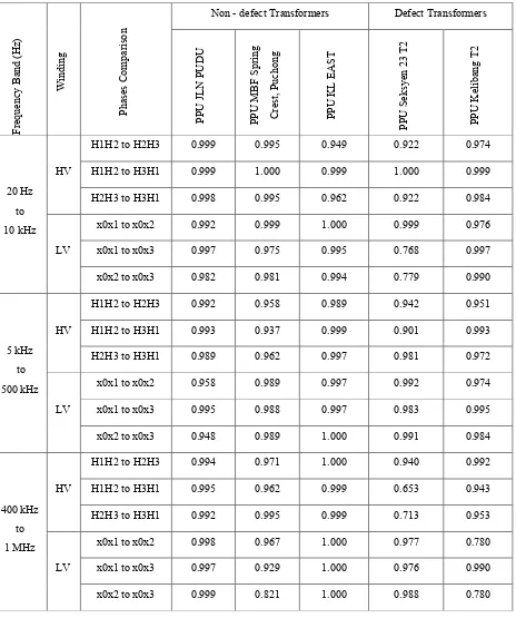
Table 2.1: Data SFRA from transformers Fre qu en cy B an d (Hz) W in din g Ph ases C om par is on

Non - defect Transformers Defect Transformers

PP U JL N PUDU PP U MB F Sp rin g C rest, Pu ch on g PP U KL E AST PP U Sek sy en 2 3 T2 PP U Kelib an g T2 20 Hz to 10 kHz HV

H1H2 to H2H3 0.999 0.995 0.949 0.922 0.974

H1H2 to H3H1 0.999 1.000 0.999 1.000 0.999

H2H3 to H3H1 0.998 0.995 0.962 0.922 0.984

LV

x0x1 to x0x2 0.992 0.999 1.000 0.999 0.976

x0x1 to x0x3 0.997 0.975 0.995 0.768 0.997

x0x2 to x0x3 0.982 0.981 0.994 0.779 0.990

5 kHz to 500 kHz

HV

H1H2 to H2H3 0.992 0.958 0.989 0.942 0.951

H1H2 to H3H1 0.993 0.937 0.999 0.901 0.993

H2H3 to H3H1 0.989 0.962 0.997 0.981 0.972

LV

x0x1 to x0x2 0.958 0.989 0.997 0.992 0.974

x0x1 to x0x3 0.995 0.988 0.997 0.983 0.995

x0x2 to x0x3 0.948 0.989 1.000 0.991 0.984

400 kHz to 1 MHz

HV

H1H2 to H2H3 0.994 0.971 1.000 0.940 0.992

H1H2 to H3H1 0.995 0.962 0.999 0.653 0.943

H2H3 to H3H1 0.992 0.995 0.999 0.713 0.953

LV

x0x1 to x0x2 0.998 0.967 1.000 0.977 0.780

x0x1 to x0x3 0.997 0.929 1.000 0.976 0.990

(19)

This tool Self Organizing Map using Euclidean distance formula to calculate distance for each neurons that to be train by the SOM where the distance between two point in the grid with their coordinate estimate (X,Y) and (A,B) as:

�� , , , = (X−A)2_{+ (Y}−_B)2

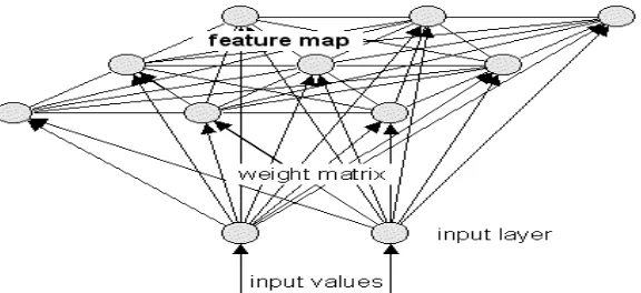
Very often, especially when measuring the distance in the plane, we use the formula for the Euclidean distance. According to the Euclidean distance formula, the distance between two points in the plane with coordinates (x, y) and (a, b) is given as illustrated in figure 2.1.

Figure 2.1: Result from SOM.

Figure 2.2: Result from SOM1.

(20)

contain variable value will present to neuron and it make neuron attempt to become like input data.

The neuron that receives data will adjust their weights along data value where it called as training. This neuron will train data several time and each time data input to neuron it call epoch. This process will continuously loop and the data input given will change the neuron and it will train again to get a pattern and it will give result as a topographic map.

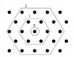
The neuron have a connection between them with the relation by neighborhood where it response each other by weight and distance. These topology structures have two type of factor which is local lattice structure and global map where in this project it uses local lattice structure as figure 2.3 below.

Figure 2.3: Hexagonal lattice.

Using hexagonal lattice is better than others in this project because it have the most plot of weight in their neighbor, this characteristic of structure can produce an accurate data to perform the diagnosis.

The data that provided need to be brought in Matlab by using standard M file , this will be perform by calling the data using command which it can be seen in appendix. In this project, the node or each neuron is representative a data from FRA. Every time data change it will affect the output at SOM and it will follow the data input given.

(21)

This normalizing is important because it can protect the data from overwhelming and hold the data to repeat the normalization or denormalize. The simple instruct command can be seen in appendix. The data had been normalize and it need to initialization and been train, there are two type of initialization which is random and linear algorithm. This initialization can be perform in simple command which is it can be seen in appendix.

2.3 Summary of Literature Review

(22)

METHODOLOGY

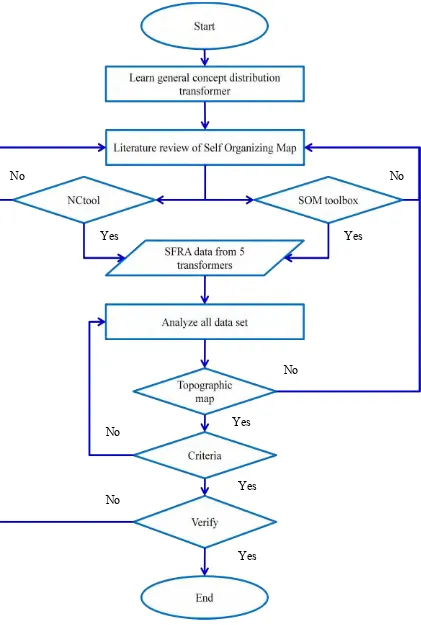
3.1 Introduction of Methodology

(23)

Figure 3.1: Flow chart of methodology. Yes

No No

Yes

No

(24)

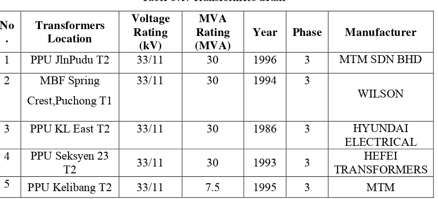
distribution transformer had been learning. In this research it focuses on the data from SFRA where the data is important to determine the good or bad transformer. This research work using five TNB transformers specification data as the input data for Self Organizing Map method to analyze and intemperate the data in visual mode using topographic map. In table 3.1 represent details transformers of the distribution transformers that being used in this research work.

Table 3.1: Transformers detail

No . Transformers Location Voltage Rating (kV) MVA Rating (MVA)

Year Phase Manufacturer

1 PPU JlnPudu T2 33/11 30 1996 3 MTM SDN BHD 2 MBF Spring

Crest,Puchong T1

33/11 30 1994 3

WILSON

3 PPU KL East T2 33/11 30 1986 3 HYUNDAI ELECTRICAL 4 PPU Seksyen 23

T2 33/11 30 1993 3 TRANSFORMERS HEFEI 5 PPU Kelibang T2 33/11 7.5 1995 3 MTM