PRESENTASI
SOAL dan
JAWABAN
Question 1
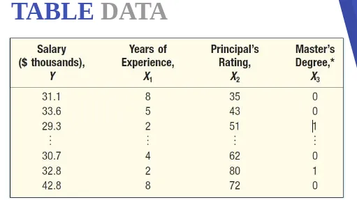
Mike Wilde is president of the teachers’ union for Otsego School
District. In preparing for upcoming negotiations, he would like to
investigate the salary structure of classroom teachers in the district. He believes there are three factors that affect a teacher’s salary: years
of experience, a rating of teaching effectiveness given by the principal, and whether the teacher has a master’s degree. A random
TABLE
DATA
Develop a correlation matrix. Which independent variable has the strongest correlation with the dependent variable? Does it appear there will be any problems with multicollinearity?
Strongest Correlation: => Salary with Years of Experience
Salary Experience, XYears of
1
Principal’s
Rating, X2 Master's Degree
Salary 1
Years of
Experience, X1 0,577299 1 Principal’s
Rating, X2 0,442869 -0,32744 1
Master's Degree -0,37181 -0,80861 0,373321 1
Determine the regression equation. What salary would you estimate for a teacher with five years experience, a rating by the principal of 60, and no masters
degree?-last-▸ Regression Equation:
Conduct a global test hypothesis to determine whether any of the regression coefficients differ from zero. Use the .05 significance level.
Bring the attention of your audience over a key concept using icons or
Conduct a test of hypothesis for the individual regression coefficients. Would you consider
deleting any of the independent variables? Use the .05 significance level.
▸ Using the regression table, the t ratio of years experience is 1,5131 and the p values of Years experience is 0.2694. Because the p value is more than 0.05, we conclude that the years expereince regression coefficient could equal 0. Thus, years of experience should not be included in the equation to predict a teacher’s salary.
▸ The t ratio of principal’s rating is 1,9658 and the p value is 0,1882. The p value is more than 0.05 the principal rating could equal 0. So, principal’s rating should not be included in the equation topredict teachers salary.
▸ The t ratio of master degree is 0,0952 and the p value is 0,9328. The p value
If your conclusion in part (d) was to delete one or more independent variables, run
the analysis again without those variables.
E.
SUMMARY OUTPUTRegression 2 92,21767238 46,10883619 5,334477 0,102820327 Residual 3 25,93066095 8,643553651
Total 5 118,1483333
F.
Question 2 - 44
▸ A sample of 12 homes sold last week in St. Paul, Minnesota,
a. Compute the correlation coefficient.
Home Size Selling Price
Mean 1,15 Mean 96,66666667 Standard Error 0,054355731 Standard Error 4,536607552
Median 1,15 Median 102,5 Mode 1,1 Mode 105 Standard Deviation 0,188293774 Standard Deviation 15,71526955
Sample Variance 0,035454545 Sample Variance 246,969697 Kurtosis -0,488888889 Kurtosis -0,943584629 Skewness -0,39218585 Skewness -0,453624695
Range 0,6 Range 50 Minimum 0,8 Minimum 70 Maximum 1,4 Maximum 120
a. Compute the correlation coefficient.
Home Size Selling Price X - X Y - Y (X - X)(y - y) 1,4 100 0,25 3,333333333 0,833333333 1,3 110 0,15 13,33333333 2
1,2 105 0,05 8,333333333 0,416666667 1,1 120 -0,05 23,33333333 -1,166666667 1,4 80 0,25 -16,66666667 -4,166666667
1 105 -0,15 8,333333333 -1,25 1,3 110 0,15 13,33333333 2
0,8 85 -0,35 -11,66666667 4,083333333 1,2 105 0,05 8,333333333 0,416666667 0,9 75 -0,25 -21,66666667 5,416666667 1,1 70 -0,05 -26,66666667 1,333333333 1,1 95 -0,05 -1,666666667 0,083333333
a. Compute the correlation coefficient.
Correlation Coefficient :
b. Determine the coefficient of determination.
▸ The relationship is positive or direct, because the sign of
the correlation coefficient is positive. As the size of the home (reported in thousands of square feet) increases, the selling price (reported in $ thousands) also increases
c. Can we conclude that there is a positive
association between the size of the home and the selling price? Use the .05 significance level.
H0 is rejected. There is a positive association