APPLICATION OF SWALLOWTAIL CATASTROPHE THEORY TO TRANSIENT STABILITY ASSESSMENT OF MULTI-MACHINE POWER SYSTEM.

(1)

APPLICATION OF SWALLOWTAIL CATASTROPHE

THEORY TO TRANSIENT STABILITY ASSESSMENT OF

MULTI-MACHINE POWER SYSTEM

1_{BUGIS I .,} 2_{MAITHEM HASSEN KAREEM}

1,2_{Department of electrical engineer, Universiti Teknikal Malaysia Melaka}

E-mail: 1ismadi@utem.edu.my, 2maythem.hk@gmail.com

ABSTRACT

Transient stability analysis is an important part of power planning and operation. For large power systems, such analysis is very demanding in computation time. On-line transient stability assessment will be necessary for secure and reliable operation of power systems in the near future because systems are operated close to their maximum limits. In this manuscript swallowtail catastrophe is used to determine the transient stability regions. The bifurcation set represents the transient stability region in terms of the power system transient parameters bounded by the transient stability limits. The transient stability regions determined are valid for any changes in loading conditions and fault location. The system modeling is generalized such that the analysis could handle either one or any number of critical machines. This generalized model is then tested on numerical examples of multi-machine power system (Cigre seven machine systems) shown very good agreement with the time solution in the practical range of first swing stability analysis. The method presented fulfills all requirements for on-line assessment of transient stability of power system

Keywords: Swallowtail Catastrophe Theory, Distributed Generators, Generator Critical, Large Power

System, Transient Stability Assessment.

1. INTRODUCTION

A stable power system implies that all its interconnected generators are operating in synchronism with each other and the rest of power system network. Problems arise when the generators oscillate because of disturbances that occur from transmission faults or load switching operations. The stability problem of power system has been given new importance since the famous blackout in Northeast U.S.A. in 1965[7]. Considerable research effort has gone into the stability investigation both for off-line and on-line purposes. Since then a stringent rules on Operation and Control procedures of electric power systems are imposed. It started a chain reaction affecting planning. There are two types of stability problem in power systems. Firstly, the steady state stability problem which refers to the stability of power systems when a small disturbance occurs in the power systems such as a gradual change in loads, manual or automatic changes in excitation irregularities in prime-mover input. Obviously these kind of disturbance never lead to loss of synchronism unless the system is operating at, or very near to, its steady state stability boundary. This boundary is the greatest power that can be

(2)

brought back to synchronism. While this can be done readily with gas and water turbine generators, steam turbine generators require many hours to rebuild steam and the operator has to shed load to compensate for the loss of generators. Loss of synchronism may also cause some protective relays to operate falsely and trip the circuit breakers of unfaulted lines. In such cases the problem becomes very complicated and may result in more generators losing synchronism. Therefore, transient stability of power systems becomes a major factor in planning and day-to-day operations and there is a need for fast on-line solution of transient stability to predict any possible loss of synchronism and to take the necessary measures to restore stability. Since then several studies have been conducted and new concepts and directions have been suggested to prevent instability and ensure security and reliability of power systems such as direct method Lyapunov's and pattern recognition which have been introduced for fast assessment of transient stability and eventually to implement these methods for on-line applications. Catastrophe theory has been pragmatic to the study of stability of various dynamic systems [2] and in recent years to the steady state stability problem of power systems by Sallam and Dineley [3]. An attractive feature of Catastrophe Theory is that the stability regions are defined in terms of the system parameters bounded by the lines of stability limits. Tavora and Smith [8] introduced Centre Of Inertia (COI) technique for multi-machines power system which has been proven to give a good result in direct stability analysis. In this manuscript swallowtail catastrophe theory has been applied to find the sudden change of generator rotor angle operation. This is recognized as operational discontinuity in concept of Catastrophe Theory. It simplifies the transient stability assessment (TSA) problem by unifying diverse stability boundaries into the operational discontinuity.

2. CATASTROHE THEORY

It is a natural phenomenon that sudden changes can occur as a result of smooth or gradual changes. Examples might include the breakdown of an insulator when voltage is built up gradually, the collapse of a bridge by gradual load increases and the loss of synchronism of generators in a power system when subject to smooth changes in operating conditions. The term "catastrophe" is used for such sudden changes that are caused by smooth alterations.

The foundations of catastrophe theory were developed by the French mathematician

Rene'Thorn and became widely known through his book Stabilite' Structurelleet Morphogenese [14] in which he proposed them as a foundation for biology. A catastrophe, in the very broad sense Thom gives to the world, is any discontinuous change that occurs when a system perhaps have more than one stable case, or can follow more than one stable pathway of change. The catastrophe is the jump from one case or pathway to other [5]. The elementary catastrophes are the seven simplest ways such a transaction from one state to another state can occur. This is true for any system governed by a potential, and in which the manners of the system is determined by less than five different factors, then only seven qualitatively diverse types of discontinuity are possible [6] .The qualitative type of any stable discontinuity does not depend on the specific nature of the potential involved, merely on its existence, i.e. on the existence of cause-and-effect relationship between conditions. Now we can see how the elementary catastrophes are comparable to the regular forms of classical geometry. Just as we can say that any three dimensional object, if it is regular (i.e. all its faces are identical polygons ), must be one of the five solids, so the catastrophe theory asserts that any discontinuous process whose behavior can be described by a graph in as many as six dimensions, if structurally stable, must correspond to one of the seven elementary catastrophes [9] .This manuscript generalizes the use of catastrophe theory to the case of multi-machine power systems, with more than one machine being critical (likely to go unstable). The mathematical ideas involved in reducing the multi-machine power system and the application of catastrophe theory by (seven machine cigre system). In deriving the equations for the multi-machine system, the general dynamic equivalent approach is used, grouping all the critical generators as one equivalent machine and grouping the rest of the system as another single equivalent machine.

Consider a continuous potential function V(x,c) which represents the system behavior, where x are the state variables and c are the control parameters. The potential function V(x,c) can be mapped in terms of its control variables c to define the continuous region. Let the potential function be represented as:

V(x,c) : M

⊗

R (1)

(3)

surface that represents all critical points of V(x,c).

It is the subset

R

n

×

R

rdefined by:

( ) x

V

c x

∇

(2)

Where Vc(x) = V(x,c) and is partial derivative with respect to x. Equation (2) is the set of all critical points of the function V(x,c). Next we find the singularity set, S, which is the subset of M that focus on all degenerate critical points of V. It is defined by :

( ) x

V

c x

∇

And

2 (x) x

V

c

∇

(3)

The singularity set, S, is then projected down onto the control space Rr by eliminating the state variables x using equations (2) and (3), to obtain the bifurcation set, B. The bifurcation set provides a projection of the stability region of the function V(x,c), i.e. it contains all non-degenerate critical points of the function V bounded by the degenerate critical point at which the system exhibits sudden changes when it is subject to small changes of control parameters.

Figure (1) p-δ curve and equal area criteria [10]

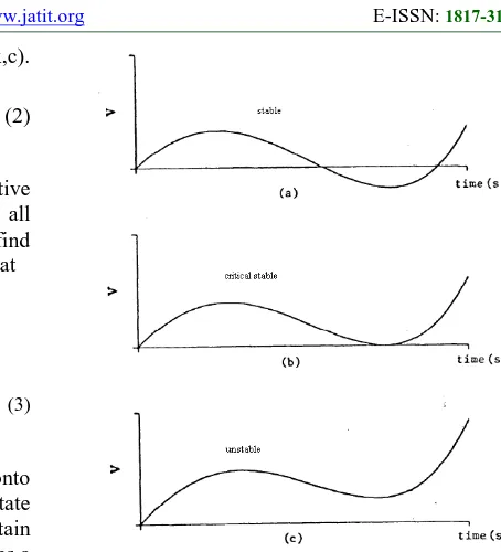
Figure (1) showing power-angle area if a fault occurs on one of the transmission lines near the generator bus. The rotor will start to accelerate and hence the machine would gain kinetic energy. If the fault is cleared at a clearing time such that the kinetic energy (A1) produced by the fault is absorbed by the potential energy (A2) produced after the clearance of the fault and the gained energy is less than zero then the system is stable and, if exactly zero the system is critically stable otherwise the system attend to unstable case .this is showing in figure (2)

Figure (2) energy function stability criteria [13]

2.1 Catastrophe Theoy Application In Tsa

The transient stability problem of multi-machine power system is much more complicated because the analysis of multi-machine involves individual machine in the power system without equivalencing any machine. In this case of transient stability there are two switchings (discontinuities) during the transient period, one at fault happening and the other at fault clearance. Before we attempt to apply the swallowtail catastrophe theory we need to find a continuous function that represents the system performance during the transient period. We need also to classify the degenerate and non-degenerate critical points in terms of transient stability.

[image:3.612.86.523.63.323.2] [image:3.612.285.512.74.324.2] [image:3.612.94.296.420.562.2]

(4)

n i i k

M

≠

=

∑

 (4)

1

n i i i k

M

δ

≠

=

∑

  (5)

Where

M

_ and

δ

_, respectively, inertia constant and angle of the centres of the system excluding the critical machine.

Let

k k

θ δ δ

= −

 (6)

1

(

)

n

i

k k i

i k

M

θ δ

δ

≠

= −

∑

 (7) Also

1

(

)

n i

k k i

i k

M

θ δ

δ

≠

= −

∑





(8)

1

(

)

n

i

k k i

i k

M

θ δ

δ

≠

= −

∑





( 9)

i i mi ei

M

δ =



P

−

P

(10)

1

(

cos

sin )

n

ei j

EiEj gij

ij

bij

ij

P

δ

=

=+

∑

(11)

Where:

ei

P =Electrical power output of machines

mi

P

=Mechanical power input

i

M

=Inertia constant

δ

i=Rotor angle

E

i=Internal voltage

gij

=Transfer conductance

bij

=Transfer susceptance

δ

ij

=

i

−

j

We substitute equation (10) into (9) to obtain the swing equation machine (k) with respect to the center of angle (COA)

1

(

)

n mk ek mi ei k

k i k

P

M

θ

≠

−

=

−

∑

−





(12)

Substituting equation (11) and separating

θ

_kfrom the rest of the system we get the swing equation of the critical machine (k) against the rest of the power system. This will be explained in the following steps:

Lets:

ij i j

g

ij

D

=

E E

(13)

i j

ij ij

C

=

E E

b

(14)

Equation (12) becomes:

(

cos

sin

)

cos

sin

)

cos

sin

(

k k mk k

n n

k

mi ij ij ij

i k j k

n k

ik ik ik

ik i k

n

kj kj kj kj

j k

M

P

D

M

D

C

P

ij

M

C

D

M

C

D

θ

≠ ≠ ≠ ≠

=

−

+

−

+

∑

 



(15) Lets:

(

cos

sin

)

k mk k

n n

k

mi ij ij ij

i k j k

P

D

M

D

C

P

ij

M

_≠ _≠

θ

=

−

∑

−

∑

+



(16)

Then

[ sin

cos

]

k k k

b

k

a

k

M

θ =−



P

−

θ

(17)

Where

cos

sin

)

sin

cos

(

n k

i ik i

ik i k n

kj

kj j j

j k

M

a

D

C

M

C

D

θ

≠ ≠

=+

−

∑

 (18) 0

sin

cos

)

sin

cos

)

(

n

j ij j

kj j k

n k

i ik i

ik i k

b

D

C

M

D

C

M

θ

≠ ≠

=+

−

∑

(19)

Equation (17) can be written in a more convenient from :

sin(

)

k k k k k k

M

δ



−

=

P

T

−

θ α

(20)

Where

1

( )

tan

k

a

b

(5)

2 2

k

a

b

T

=

+

(22)

Equation (20) is a simple form representing the motion of the critical machine for a certain disturbance. Since we assumed that the rest of the system is not responding to the disturbance, it is reasonable to use the pre-disturbance angle

θ

_ to

calculate the parameters

P

_k ,

T

_k and

α

_k . the stable and unstable equilibrium points of equation (20) can be easily computed by solving equation (23).

sin(

s

)

0

k k k k

P

−

T

θ α

−

=

(23) And the unstable equilibrium point (UEP) is

u s

k

π

k

θ

= −

θ

(24) We note here that we have two sets of the parameters

P

_k,

T

_kand

α

_k; one set for the fault-on network and another for the post-fault network. Multiplying equation (20) by

θ



_kand integration

between

θ

c_kand

θ

_k° with respect to time for the fault-on network parameters we obtain the kinetic energy generated by the fault.

(

)

[cos(

)

cos(

)]

f c f f

k k k

f c

k k

kin

P

θ θ

T

θ α

θ θ

° °

=

−

(25)

Where

P

_kf ,

T

_kf and

α

_kf are the system parameters for fault-on network and

θ

c_k is the clearing angle . The potential energy of the post-fault network is derived in the same approach by integrating

equation (20) between

θ

c_kand

θ

u_k using the post-fault network parameter , we obtain :

(

)

[cos(

)

cos(

)]

f u c p c p

k k k

p u

k k

pot

P

θ θ

T

θ α

=

−

(26)

So, the energy balance equation for critical clearing becomes:

2

1

cos(

)

0

2

p p p

c c c u

k k

k k k

M

θ

−

P

θ

−

T

θ α

−

+

D

=

(27) Where

cos(

)

p p

u u P c

k

k k

N

= +

P

θ

T

−

θ θ

(28) We represent c

k

θ

by Taylor Series expansion

2

(

)

sin(

)

c c f

M

t

Pm

P

θ θ

θ

−

=

−

  (29) 2

1

2

c k

k k

Y

t

c

θ θ

= +



(30)

Where

1

[

( )]

k k e

k

t

Y

P

M

=

−

(31)

Let

1

2

k c

x

=

Y

t

By replacing

cos(

θ

α

P

)

R C

R

−

in equation (27) with

cosine series expansion up to the fourth order, we get:

2

4

(

)

(

)

[1

2!

(

)

0

4!

p

p p x k

k k k k

p k

x u

x

M

Y

x

P

x

T

x

D

α

θ

α

θ

+ −

−

+ −

−

+ −

+

+ =



(32)

Let

β

=

(

θ



_k

−

α



_k

)

Then we get catastrophe theory manifold equation Let: 3 2 2 3 1 2 4

4

12(1

)

2

24

(

)

6

24

(

)

2

24

p

p p k

k k k

p k

p p

p p p k k

u

k k k

p k

A

T

M

A

Y

P

T

N

A

T

P

T

β

θ

°

= −

=

−

= −

−

+

−

= −

− −

+

−

and

x

= −

y

µ

3

4

A

µ

=

We obtain the swallowtail catastrophe manifold

4 2

0

u

vy

w

y

+

y

+ + =

(33) Where 2 2 3

3

(

)

8

u

=

A

−

A

(34)

3 3 2 3 1

(

)

2

8

A A

A

v

=

A

−

+

(35)

2 4

1 3 2 3

3

(

)

4

16

256

A A

A

(6)

3. NUMERICAL EXAMPLE

Table 1: (Tcc) Estimation By Proposed Method Is Tabulated As:

Figure(3) Cigre seven machine system

A Cigre seven bus system show in figure (3) [see Appendix to its data] was used as the system examination. The perturbation is simulated as a fault occur on the Transmission line. Simulation was performed in a numerous times to get the approximate critical clearing time (CCT). The (CCT) estimation by suggested method is tabulated in table (1). As following

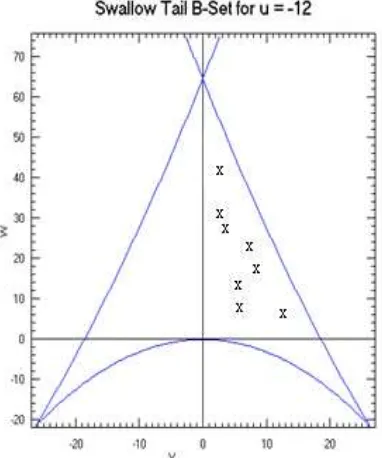
Figure (4): bifurcation set of swallowtail

The importance of the transient stability regions provided by the bifurcation set of the catastrophe manifold is not only in terms of speed and accuracy. It provides another important dimension to the transient stability problem-the stability limits. The method checks for the violations of the transient stability limits of the post-fault network in terms of the system parameters. Of course, if the

Fault at Bus TCC simulation

TCC Proposed

method

1 0.36 0.36

2 0.41 0.37

3 0.39 0.39

4 0.50 0.48

5 0.35 0.35

6 0.52 0.51

7 0.33 0.33

(7)

limits are exceeded the system is unstable. This important feature is not possible with existing direct methods, i.e., the existing direct methods cannot give any solution when the stability limits of the post-fault network are violated. To obtain good accuracy beyond this limit higher order terms have to be included in the computations. This will complicate the stability region and slow down the calculation procedure. In practice, however, this problem is very rare. Faults in large power systems are usually tripped in a few cycles, typically in range 0.1-0.3 seconds. Interest is in the delivery of maximum power at low clearing time without risking the power system security. This practical consideration can easily be handled by the proposed method without loss of accuracy.

4. CONCLUSION

This manuscript suggest a method to solve the transient stability problem of multi-machine power Systems with the system having more than one critical machine for a specified disturbance. Here the critical machines during a three-phase fault are identified, single-out and combined to be one equivalent machine and also the rest of the system as another single equivalent machine using the general dynamic equivalent approach. Then the energy balance equation is derived from the equation of motion of the equivalent critical machine against the rest of the system. The energy balance equation is then used to form the equilibrium surface of the swallowtail catastrophe manifold from which the transient stability region is derived by the bifurcation technique. The results obtained by this general swallowtail catastrophe approach is in good agreement with those obtained by the time solution method.

ACKNOWLEDGEMENT

Authors would like to thank the encouragement and financial assistance of Malaysia government (KPT grant FRGS/1/2102/TK02/UTEM/02/5) and UniversitiTeknikal Malaysia Melaka (UTeM) as well as Laboratory Researchers of the UTeM for their support

REFRENCES:

[1] E.W. Kimbark, "Power System Stability", Vol. I, John Wiley & Sons Inc., New York, 1948.

[2] T. Poston and I. Stewart, Catastrophe Theory

and Its Applications,Pitman Publishing Co.,

London, 1979.

[3] A.A. Sallam and J.L. Dineley, Catastrophe

theory as a Tool for Determining Synchronous Power System Dynamic Stability , IEEE Trans.

PAS, Vol. 102, pp. 622-630, March 1983. [4] P. Saunders, "An Introduction to Catastrophe

Theory,". Cambridge University Pres 1980

[5] C. Panati, "Catastrophe theory," Newsweek, January 19, 1976.

[6] M. Davis and A. Woodcock, "Catastrophe

Theory,". Clarke, Irwin and Company Limited,

Toronto, 1978.

[7] E. W. Kimbark, Power System Stability, Vol. 1. John Wiley and Sons Inc., New York,1984 [8] Tavora, C.J.; Smith, O.J.M., Characterization

of Equilibrium and Stability in Power Systems, Power Apparatus and Systems, IEEE

Transactions on , vol.PAS-91, no.3,

pp.1127,1130, May 1972

[9] I. Stewart and T.Poston, "Catastrophe Theory

and its Applications,".Pitman Publishing,

Londo,1979.

[10] Zhenhua Wang; Aravnthan, V.; Makram, E.B.,

Generator cluster transient stability assessment using catastrophetheory,Environment and Electrical Engineering (EEEIC),2011 10th

International Conference on , vol., no., pp.1,4, 8-11 May 2011

[11] Y. Xue, Th. Van. Cutsem and Ribbens-Pauella,

"A Simple Direct Method for Fast Transient Stability Assessment of Large Power Systems",

IEEE PES Winter Meeting, New Orleans, Louisiana, February 1-6, 1987.

[12] A.N. Michel, A.A. Fouad and V. Vittal , "Power System Transient Stabilitby Using

Individual Machine Energy Functions", IEEE

Trans., CAS-30, May 1983, pp. 266-276. [13] H. Hakkimmashhadi, "Fast Transient Stabilit

y Assessment", Ph.D. thesis, Purdue University,

West Lafayette, Indiana, Aug. 1982.

[14] R.Thorn, "Structural Stability and

Morphogenesis", Benjamin-Addison Wesley,

New York, 1975.

(8)

Line Data Of Cigre Seven Machine System

Line

From bus

To bus

R (pu)

X (pu)

BC/2(pu)

1 2 3 0.045 0.1236 0.1013

2 1 3 0.0099 0.0484 0.1013

3 3 4 0.0119 0.078 0.1519

4 4 10 0.0164 0.0652 0.1519

5 4 1 0.009 0.0484 0.0506

6 8 6 0.0188 0.0628 0.1013

7 4 6 0.0075 0.0198 0.6075

8 4 5 0.0039 0.0198 0.1013

9 2 10 0.0164 0.0638 0.0152

10 9 8 0.0488 0.1916 0.1013

11 9 4 0.0488 0.1916 0.1013

12 3 9 0.0115 0.0553 0.1013

13 8 7 0.0119 0.078 0.1519

Bus Data Of Cigre Seven Machine System

BUS

TYPE Magnitude

voltage Angle PG(PU) QG(PU) PL(PU) QL(PU)

1 PV 1.0611 6.11984 2.13832 0.564363 0 0

2 SWING 1.0051 0 1.38105 1.11728 2 1.2

3 PV 1.047 4.69996 2.53843 0.707422 0 0

4 PV 1.0254 2.47471 2.88663 1.62199 6.5 4.05

5 PV 1.0507 4.71052 2.30594 0.817952 0 0

6 PV 1.0322 2.79355 1.57806 0.0370282 0.8 0.3

7 PV 1.0195 5.27133 1.72832 0.290893 0.9 0.4

8 PQ 1.00806 1.69941 -0.003658 0 1 0.5

9 PQ 0.974951 -0.327217 -0.001181 -0.001963 2.3 1.4

10 PQ 0.998046 -0.273962 0.0002112 -0.000403 0.9 0.45

Generator Data Of Cigre Seven Machine System

Gen Bus H (pu) D (pu) Xq′ (pu) Td′ Tq′ E (pu)

δ

(degree)

1 1 24.08 0 0.074 8.96 0.4 1.11052 13.837

2 2 16.44 0 0.118 6 0.535 1.14778 8.12087

3 3 30.36 0 0.124 5.89 0.6 1.17006 19.5885

4 4 38.16 0 0.049 5.89 0.6 1.1115 9.60369

5 5 24.08 0 0.074 8.96 0.4 1.12014 13.047

6 6 27.08 0 0.071 6 0.535 1.04042 8.78211