An Extended ID3 Decision Tree Algorithm for
Spatial Data
Imas Sukaesih Sitanggang#†1, Razali Yaakob#2, Norwati Mustapha#3, Ahmad Ainuddin B Nuruddin*4
#
Faculty of Computer Science and Information Technology, Universiti Putra Malaysia 43400 Serdang Selangor, Malaysia
1
[email protected], [email protected], [email protected] *
Institute of Tropical Forestry and Forest Products (INTROP), Universiti Putra Malaysia 43400 Serdang Selangor, Malaysia
4
†Computer Science Department, Bogor Agricultural University, Bogor 16680, Indonesia
Abstract— Utilizing data mining tasks such as classification on spatial data is more complex than those on non-spatial data. It is because spatial data mining algorithms have to consider not only objects of interest itself but also neighbours of the objects in order to extract useful and interesting patterns. One of classification algorithms namely the ID3 algorithm which originally designed for a non-spatial dataset has been improved by other researchers in the previous work to construct a spatial decision tree from a spatial dataset containing polygon features only. The objective of this paper is to propose a new spatial decision tree algorithm based on the ID3 algorithm for discrete features represented in points, lines and polygons. As in the ID3 algorithm that use information gain in the attribute selection, the proposed algorithm uses the spatial information gain to choose the best splitting layer from a set of explanatory layers. The new formula for spatial information gain is proposed using spatial measures for point, line and polygon features. Empirical result demonstrates that the proposed algorithm can be used to join two spatial objects in constructing spatial decision trees on small spatial dataset. The proposed algorithm has been applied to the real spatial dataset consisting of point and polygon features. The result is a spatial decision tree with 138 leaves and the accuracy is 74.72%.
Keywords—ID3 algorithm, spatial decision tree, spatial information gain, spatial relation, spatial measure
I. INTRODUCTION
Utilizing data mining tasks on a spatial dataset differs with the tasks on a non-spatial dataset. Spatial data describe locations of features. In a non-spatial dataset especially for classification, data are arranged in a single relation consisting of some columns for attributes and rows representing tuples that have values for each attributes. In a spatial dataset, data are organized in a set of layers representing continue or discrete features. Discrete features include points (e.g. village centres), lines (e.g. rivers) and polygons (e.g. land cover types). One layer relates to other layers to create objects in a spatial dataset by applying spatial relations such as topological relations and metric relation. In spatial data mining tasks we should consider not only objects itself but also their neighbours that could belong to other layers. In addition, types of attributes in a non-spatial dataset include numerical and categorical meanwhile features in layers are represented by
geometric types (polygons, lines or points) that have quantitative measurements such as area and distance.
This paper proposes a spatial decision tree algorithm to construct a classification model from a spatial dataset. The dataset contains only discrete features: points, lines and polygons. The algorithm is an extension of ID3 algorithm [1] for a non-spatial dataset. As in the ID3 algorithm, the proposed algorithm uses information gain for spatial data, namely spatial information gain, to choose a layer as a splitting layer. Instead of using number of tuples in a partition, spatial information gain is calculated using spatial measures. We adopt the formula for spatial information gain proposed in [2]. We extend the spatial measure definition for the geometry type points, lines and polygons rather than only for polygons as in [2].
The paper is organized as follows: introduction is in section 1. Related works in developing spatial decision tree algorithms are briefly explained in section 2. Section 3 discusses spatial relationships. We explain a proposed spatial decision tree algorithm in section 4. Finally we summarize the conclusion in section 5.
II. RELATED WORKS
The works in developing spatial data mining algorithms including spatial classification and spatial association rules continue growing in recent years. The discovery processes such as classification and association rules mining for spatial data are more complex than those for non-spatial data, because spatial data mining algorithms have to consider the neighbours of objects in order to extract useful knowledge [3]. In the spatial data mining system, the attributes of the neighbours of an object may have a significant influence on the object itself.
Spatial decision trees refer to a model expressing classification rules induced from spatial data. The training and testing records for this task consist of not only object of interest itself but also neighbours of objects. Spatial decision trees differ from conventional decision trees by taking account implicit spatial relationships in addition to other object attributes [4]. Reference [3] introduced an algorithm that was designed for spatial databases based on the ID3 algorithm [1]. The algorithm considers not only attributes of the object to be
___________________________________ 978-1-4244-8351-8/11/$26.00 ©2011 IEEE
classified but to consider also attributes of neighbouring objects. The algorithm does not make distinction between thematic layers and it takes into account only one spatial relationship [4]. The decision tree from spatial data was also proposed as in [5]. The approach for spatial classification used in [5] is based on both (1) non-spatial properties of the classified objects and (2) attributes, predicates and functions describing spatial relation between classified objects and other features located in the spatial proximity of the classified objects. Reference [6] discusses another spatial decision tree algorithm namely SCART (Spatial Classification and Regression Trees) as an extension of the CART method. The CART (Classification and Regression Trees) is one of most commonly used systems for induction of decision trees for classification proposed by Brieman et. al. in 1984. The SCART considers the geographical data organized in thematic layers, and their spatial relationships. To calculate the spatial relationship between the locations of two collections of spatial objects, SCART has the Spatial Join Index (SJI) table [7] as one of input parameters. The study [2] extended the ID3 algorithm [1] such that the new algorithm can create a spatial decision tree from the spatial dataset taking into account not only spatial objects itself but also their relationship to its neighbour objects. The algorithm generates a tree by selecting the best layer to separate a dataset into smaller partitions as pure as possible meaning that all tuples in partitions belong to the same class. As in the ID3 algorithm, the algorithm uses the information gain for spatial data, namely spatial information gain, to choose a layer as a splitting layer. Instead of using number of tuples in a partition, spatial information gain is calculated using spatial measures namely area [2].
III. SPATIAL RELATIONSHIP
Determining spatial relationships between two features is a major function of a Geographical Information Systems (GISs). Spatial relationships include topological [8] such as overlap,
touch, and intersectand metric such as distance. For example, two different polygon features can overlap, touch, or intersect
each other. Spatial relationships make spatial data mining algorithms differ from non-spatial data mining algorithms. Spatial relationships are materialized by an extension of the well-known join indices [7]. The concept of join index between two relations was proposed in [9]. The result of join index between two relations is a new relation consisting of indices pairs each referencing a tuple of each relation. The pairs of indices refer to objects that meet the join criterion. Reference [7] introduced the structure Spatial Join Index (SJI) as an extended the join indices [9] in the relational database framework. Join indices can be handled in the same way than other tables and manipulated using the powerful and the standardized SQL query language [7]. It pre-computes the exact spatial relationships between objects from thematic layers [7]. In addition, a spatial join index has a third column that contains spatial relationship, SpatRel, between two layers. Our study adopts the concept of SJI as in [7] to store the relations between two different layers in spatial database. Instead of spatial relationship that can be numerical or
Boolean value, the quantitative values in the third column of SJI are spatial measure of features as results from spatial relationships between two layers.
We consider an input for the algorithm a spatial database as a set of layers L. Each layer in L is a collection of geographical objects and has only one geometric type that can be polygons, or lines or points. Assume that each object of a layer is uniquely identified. Let Lis a set of layers, Liand Lj
are two distinct layers in L. A spatial relationship applied to Li
and Lj is denoted SpatRel(Li, Lj) that can be topological
relation or metric relation. For the case of topological relation, SpatRel(Li, Lj) is a relation according to the dimension
extended method proposed by [10]. While for the case of metric relation, SpatRel(oi, oj) is a distance relation proposed
by [11], where oiis a spatial object in Liand oj is a spatial
object in Lj.
Relations between two layers in a spatial database can result quantitative values such as distance between two points or intersection area of two polygons in each layer. We denote these values as spatial measures as in [2] that will be used in calculating spatial information gain in the proposed algorithm. For the case of topological relation, the spatial measure of a feature is defined as follows. Let Liand Ljin a set of layersL,
Li /j, for each feature ri in R = SpatRel(Li, Lj), a spatial
measure of ridenoted by SpatMes(ri) is defined as
1. Areaof ri, if < Li, in, Lj> or < Li, overlap, Lj> hold for
all features in Liand Ljrepresented in polygon
2. Countof ri, if < Li, in, Lj> holds for all features in Li
represented in point and all features in Ljrepresented
in polygon.
For the case of metric relation, we define a distance function from p to q as dist(p, q), distance from a point (or line) p in Li
to a point (or line) q in Lj.
Spatial measure of R is denoted by SpatMer(R) and defined as SpatMes(R) = f(SpatMes(r1), SpatMes(r2), …, SpatMes(rn))
(1) for riin R, i = 1, 2, …, n and n number of features in R. f is an
aggregate function that can be sum, min, max or average. A spatial relationship applied to Liand LjinLresults a new
layer R. We define a spatial join relation (SJR) for all features p in Liand q in Ljas follows:
SJR = {(p, SpatMes(r), q | r is a feature in R associated to p
and q}. (2)
IV. EXTENDEDID3 ALGORITHM FOR SPATIAL DATA
A spatial database is composed of a set of layers in which all features in a layer have the same geometry type. This study considers only discrete features include points, lines and polygons. For mining purpose using classification algorithms, a set of layers that divided into two groups: explanatory layers and one target layer (or reference layer) where spatial relationships are applied to construct set of tuples. The target layer has some attributes including a target attribute that store target classes. Each explanatory layer has several attributes. One of the attributes is a predictive attribute that will classify tuples in the dataset to target classes. In this study the target attribute and predictive attributes are categorical. Features
(polygons, lines or points) in the target layer are related to features in explanatory layers to create a set of tuples in which each value in a tuple corresponds to value of these layers. Two distinct layers are associated to produce a new layer using a spatial relationship. Relation between two layers produces a spatial measure (1) for the new layer. Spatial measure then will be used in the formula for spatial information gain.
Building a spatial decision tree follows the basic learning process in the algorithm ID3 [1]. The ID3 calculates information gain to define the best splitting layer for the dataset. In spatial decision tree algorithm we define the spatial information gain to select an explanatory layer L that gives best splitting the spatial dataset according to values of predictive attribute in the layer L. For this purpose, we adopt the formula for spatial information gain as in [2] and apply the spatial measure (1) to the formula.
Let a dataset D be a training set of class-labelled tuples. In the non-spatial decision tree algorithm we calculate probability that an arbitrary tuples in D belong to class Ciand
it is estimated by |Ci,D|/|D| where |D| is number of tuples in D
and |Ci,D| is number of tuples of class Ciin D [12]. In this
study, a dataset contains some layers including a target layer that store class labels. Number of tuples in the dataset is the same as number of objects in the target layer because each tuple will be created by relating features in the target layer to features in explanatory layers. One feature in the target layer will exactly associate with one tuple in the dataset. For simplicity we will use number of objects in the target layer instead of using number of tuples in the spatial dataset. Furthermore in a non-spatial dataset, target classes are discrete-valued and unordered (categorical) and explanatory attributes are categorical or numerical. In spatial dataset, features in layers are represented by geometric type (polygons, lines or points) that have quantitative measurements such as area and distance. For that we calculate spatial measures of layers (1) to replace number of tuples in a non-spatial data partition.
A. Entropy
Let a target attribute C in a target layer S has l distinct classes (i.e. c1, c2, …, cl), entropy for S represents the
expected information needed to determine the class of tuples in the dataset and defined as
)
SpatMes(S) represents the spatial measure of layer S as defined in (1).
Let an explanatory attribute V in an explanatory (non-target) layer L has qdistinct values (i.e. v1, v2, …, vq). We partition
the objects in target layer S according to the layer L then we have a set of layers L(vi, S) for each possible value viin L. In
our work, we assume that the layer L covers all areas in the layer S. The expected entropy value for splitting is given by:
))
H(S|L) represents the amount of information needed (after the partitioning) in order to arrive at an exact classification.
B. Spatial Information Gain
The spatial information gain for the layer L is given by: Gain(L) = H(S) H(S|L) (5) Gain(L) denotes how much information would be gained by branching on the layer L. The layer L with the highest information gain, (Gain(L)), is chosen as the splitting layer at a node N. This is equivalent to say that we want to partition objects according to layer L that would do the “best classification”, such that the amount of information still required to complete classifying the objects is minimal (i.e., minimum H(S|L)).
C. Spatial Decision Tree Algorithm
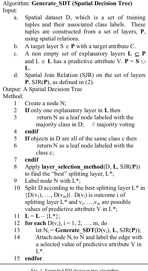
Fig. 1 shows our proposed algorithm to generate spatial decision tree (SDT). Input of the algorithm is divided into two groups: 1) a set of layers containing some explanatory layers and one target layer that hold class labels for tuples in the dataset, and 2) spatial join relations (SJRs) storing spatial measures for features resulted from spatial relations between two layers. The algorithm generates a tree by selecting the best layer to separate dataset into smaller partitions as pure as possible meaning that all tuples in partitions belong to the same class.
To illustrate how the algorithm works, consider an active fire dataset containing three explanatory layers: land cover (Lland_cover), population density (Lpopulation_density) and river
(Lriver), and one target layer (Ltarget) (Fig. 2).
Land cover layer represents polygon features for land cover
types. It has a predictive attribute that contains land cover types in the study area. They are dryland forest, paddy field, mix garden, shrubs, and paddy field (Fig. 2a).
Population layer contains polygon features for population
density. The layer has a predictive attribute population class
representing classes for population density (Fig. 2b). Classes for population density are as follows:
x Low: population_density <= 50
x Medium: 50 < population_density <= 150
x High: population_density > 150
River layer has only two attributes: the identifier of objects
and geometry representation for lines.
Target layer represents point features for true and false alarm. True alarms (T) are active fires (hotspots) and false alarms (F) are random points generated near true alarms.
The algorithm requires spatial measures in the spatial join relation (SJR) between the target layer and an explanatory layer.
Fig. 1 Extended ID3 decision tree algorithm
Table I provides spatial relationships and spatial measures we use to create SJRs.
TABLE I
SPATIALRELATION AND SPATIAL MEASURE
Target layer
Spatial Relationship
Explanatory Layer
Spatial Measure
target in land_cover count
target in population_density count target distance river distance
The spatial relationship inand the aggregate function sum
are applied to extract all objects in the target layer which are located inside land cover types (Fig. 3a) and population density classes (Fig. 3b).
The spatial relation distanceand aggregate function minare applied to calculate distance from target objects to nearest river. Distance from target objects to nearest river is represented in numerical value.
Fig. 2 A set of layers: (a) land cover, (b) population density, (c) river, (d) hotspot occurrences
Fig. 3 Target layer overlaid with (a) land cover and (b) population density
We transform minimum distance from numerical to categorical attribute because the algorithm requires categorical value for target and predictive attributes. For that, minimum distance is classified into three classes based on the following criteria:
x Low: minimum distance (km) <= 1.5
x Medium: 1.5 < minimum distance (km) <= 3
x High: minimum distance (km) > 3
Following the spatial decision tree algorithm, we start building a tree by selecting a root node for the tree. The root node is selected from the explanatory layers based on the value of spatial information gain for each layers (i.e. land cover, population density and distance to nearest river). For instance, we calculate spatial information gain for land cover
layer (Lland_cover). The same procedure can be applied to other
explanatory layers. The entropy of land cover layer for each type of land cover is given, respectively:
)) , _ (
(L _cov dryland forest C H land er
=
10 7 log 10
7 10
3 log 10
3
2
2
= 0.8812909
)) , _ (
(L _cov mix gardenC H land er
=
12 9 log 12
9 12
3 log 12
3
2
2
= 0.8112781
Algorithm: Generate_SDT (Spatial Decision Tree)
Input:
a. Spatial dataset D, which is a set of training tuples and their associated class labels. These tuples are constructed from a set of layers, P, using spatial relations.
b. A target layer S Pwith a target attribute C. c. A non empty set of explanatory layers L P
and L Lhas a predictive attribute V. P=S L.
d. Spatial Join Relation (SJR) on the set of layers
P, SJR(P), as defined in (2). Output: A Spatial Decision Tree Method:
1 Create a node N;
2 Ifonly one explanatory layer in Lthen 3 return N as a leaf node labeled with the
majority class in D; // majority voting
4 endif
5 Ifobjects in D are all of the same class c then 6 return N as a leaf node labeled with the
class c;
7 endif
8 Apply layer_selection_method(D, L, SJR(P)) to find the “best” splitting layer, L*;
9 Label node N with L*;
10 Split D according to the best splitting layer L* in {D(v1), …, D(vm)}. D(vi) is outcome i of
splitting layer L* and vi, …,vmare possible
values of predictive attribute V in L*; 11 L=L– {L*};
12 for eachD(vi), i = 1, 2, …, m, do
13 let Ni=Generate_SDT(D(vi), L, SJR(P));
14 Attach node Nito N and label the edge with
a selected value of predictive attribute V in L*.
15 endfor.
(a) (b)
(a) (b)
(c) (d)
))
From (4) we calculate the expected entropy value for splitting:
) Entropy for the target layer S:
H(S) =
From (5) we calculate the information gain for land cover
layer:
Gain(Lland_cover) = H(S) H(S|Lland_cover) = 0.352675712
The spatial information gain for other layers is as follows Gain(Lpopulation_density) = 0.18538127
Gain(Lriver) = 0.097717695
Lland_coverhas the highest spatial information gain compared to
two other layers. Therefore Lland_coveris selected as the root of
the tree. There are four possible values for land cover types: dryland forest, mix garden, paddy field, and shrubs that will be assigned as label of edges connecting the root node to internal nodes.
The Generate_SDT algorithm is then applied to a set of layer containing new explanatory layers and the target layer to construct a subtree attached to the root node. New explanatory layers are created from existing explanatory layers, best layer and the value vjof predictive attribute as a selection criterion
in a query to relate an explanatory layer and the best layer. The tree will stop growing if it meets one of the following termination criteria:
1. Only one explanatory layer in L. In this situation, the algorithm returns a leaf node labeled with the majority class in the SJR for the best layer and the explanatory layer.
2. The SJR for best layer and explanatory layer contains the same class c. Then the algorithm returns a leaf node labeled with the class c.
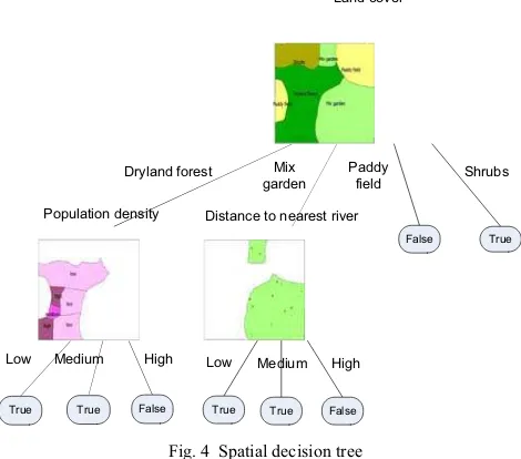
The graphical depiction of spatial decision tree generated from P = {Lland_cover, Lpopulation_desity, Lriver, target (S)} is shown
in Fig. 4. The final spatial decision tree contains 8 leaves and 3 nodes with the first test attribute is land cover (Fig. 4). Below are rules extracted from the tree:
1. IF land cover is dryland forest AND population density is low THEN Hotspot Occurrence is True
2. IF land cover is dryland forest AND population density is medium THEN Hotspot Occurrence is True
3. IF land cover is dryland forest AND population density is high THEN Hotspot Occurrence is False
Land cover
Distance to nearest river
Low High
True True False
Medium
True
Fig. 4 Spatial decision tree
4. IF land cover is mix garden AND distance to nearest river is low THEN Hotspot Occurrence is True
5. IF land cover is mix garden AND distance to nearest river is medium THEN Hotspot Occurrence is True
6. IF land cover is mix garden AND distance to nearest river is high THEN Hotspot Occurrence is False
7. IF land cover is paddy field THEN Hotspot Occurrence is False
8. IF land cover is shrubs THEN Hotspot Occurrence is True
The decision tree has the misclassi¿FDWLRQ HUURU RI WKH training set: 16.67% and the error of the testing set: 20%. The accuracy of the tree on the testing set is 80%. The number of target objects in the testing set is 30 and the number of correctly classified objects is 24.
The proposed algorithm has been applied to the real active fires dataset for the Rokan Hilir District, Riau Province Indonesia with the total area is 896,142.93 ha. The dataset contains five explanatory layers and one target layer. The target layer consists of active fires (hotspots) as true alarm data and non-hotspots as false alarm data randomly generated near hotspots. Explanatory layers include distance from target objects to nearest river (dist_river), distance from target objects to nearest road (dist_road), land cover, income source and population density for the village level in the Rokan Hilir District. Tabel II summaries the number of features in the dataset for each layer.
TABLE III
NUMBER OF FEATURES IN THEDATASET
Layer Number of features dist_river 744 points
dist_road 744 points land_cover 3107 polygons income_source 117 polygons population 117 polygons
target 744 points
The decision tree generated from the proposed spatial decision tree algorithm contains 138 leaves with the first test attribute is distance from target objects to nearest river (dist_river). The accuracy of the tree on the training set is 74.72% in which 182 of 720 target objects are incorrectly classified by the tree. Some preprocessing tasks will be applied to the real spatial dataset such as smoothing to remove noise from the data, discretization and ggeneralization in order to obtain a spatial decision tree with the higher accuracy.
V. CONCLUSIONS
This paper presents an extended ID3 algorithm that can be applied to a spatial database containing discrete features (polygons, lines and points). Spatial data are organized in a set of layers that can be grouped into two categories i.e. explanatory layers and target layer. Two different layers in the database are related using topological relationships or metric relationship (distance). Quantitative measures such as area and distance from relations between two layers are then used in calculating spatial information gain. The algorithm will select an explanatory layer with the highest information gain as the best splitting layer. This layer separates the dataset into smaller partitions as pure as possible such that all tuples in partitions belong to the same class.
Empirical result shows that the algorithm can be used to join two spatial objects in constructing spatial decision trees on small spatial dataset. Applying the proposed algorithm on the real spatial dataset results a spatial decision tree containing 138 leaves and the accuracy of the tree on the training set is 74.72%.
ACKNOWLEDGMENT
The authors would like to thank Indonesia Directorate General of Higher Education (IDGHE), Ministry of National
Education, Indonesia for supporting PhD Scholarship (Contract No. 1724.2/D4.4/2008) and Southeast Asian Regional Centre for Graduate Study and Research in Agriculture (SEARCA) for partially supporting the research.
REFERENCES
[1] J. R. Quinlan, “Induction of Decision Trees,” Machine Learning, vol. 1, Kluwer Academic Publishers, Boston, pp. 81-106, 1986.
[2] S. Rinzivillo and T. Franco, Classi¿FDWLRQ LQ *HRJUDSKLFDO
Information Systems. Lecture Notes in Artificial Intelligence. Berlin Heidelberg: Springer-Verlag, pp. 374–385, 2004.
[3] M. Ester, Kr. Hans-Peter, and S. Jörg, “Spatial Data Mining: A Database Approach,” in Proc. of the Fifth Int. Symposium on Large Spatial Databases, Berlin, Germany, 1997.
[4] K. Zeitouni and C. Nadjim, “Spatial Decision Tree – Application to Traffic Risk Analysis,” in ACS/IEEE International Conference,IEEE, 2001.
[5] K. Koperski, J. Han and N. Stefanovic, “An efficient two-step method for classification of spatial data,” In Symposium on Spatial Data Handling, 1998.
[6] N. Chelghoum, Z. Karine, and B. Azedine, “A Decision Tree for Multi-Layered Spatial Data,” in Symposium on Geospatial Theory, Processing and Applications, Ottawa, 2002.
[7] K. Zeitouni, L. Yeh, and M.A. Aufaure, “Join Indices as a Tool for Spatial Data Mining,” in International Workshop on Temporal, Spatial and Spatio-Temporal Data Mining, 2000.
[8] M. J. Egenhofer, and D. F. Robert, “Point-set topological spatial relations,” International Journal of Geographical Information Systems, vol. 5(2), pp. 161 – 174, 1991.
[9] P. Valduriez, “Join indices,” ACM Trans. on Database Systems, vol. 12(2), pp. 218-246, June 1987.
[10] E. Clementini, P. Di Felice, and O. Oosterorn, A small set of formal topological relationships suitable for end-user interaction. Lecture Notes in Computer Science. New York: Springer, pp. 277–295, 1993. [11] M. Ester, K. Hans-Peter, and S. Jörg, “Algorithms and Applications for
Spatial Data Mining,” Geographic Data Mining and Knowledge Discovery, Research Monographs in GIS, Taylor and Francis, 2001. [12] J. Han and M. Kamber, Data Mining Concepts and Techniques,2nd
ed., San Diego, USA: Morgan-Kaufmann, 2006.