Chemical Process Design and Integration
Robin Smith
Centre for Process Integration,
Chemical Process Design and Integration
Robin Smith
Centre for Process Integration,
West Sussex PO19 8SQ, England Telephone (+44) 1243 779777
Email (for orders and customer service enquiries): [email protected] Visit our Home Page on www.wileyeurope.com or www.wiley.com
All Rights Reserved. No part of this publication may be reproduced, stored in a retrieval system or transmitted in any form or by any means, electronic, mechanical, photocopying, recording, scanning or otherwise, except under the terms of the Copyright, Designs and Patents Act 1988 or under the terms of a licence issued by the Copyright Licensing Agency Ltd, 90 Tottenham Court Road, London W1T 4LP, UK, without the permission in writing of the Publisher. Requests to the Publisher should be addressed to the Permissions Department, John Wiley & Sons Ltd, The Atrium, Southern Gate, Chichester, West Sussex PO19 8SQ, England, or emailed to [email protected], or faxed to (+44) 1243 770620.
Designations used by companies to distinguish their products are often claimed as trademarks. All brand names and product names used in this book are trade names, service marks, trademarks or registered trademarks of their respective owners. The Publisher is not associated with any product or vendor mentioned in this book.
This publication is designed to provide accurate and authoritative information in regard to the subject matter covered. It is sold on the understanding that the Publisher is not engaged in rendering professional services. If professional advice or other expert assistance is required, the services of a competent professional should be sought.
Other Wiley Editorial Offices
John Wiley & Sons Inc., 111 River Street, Hoboken, NJ 07030, USA Jossey-Bass, 989 Market Street, San Francisco, CA 94103-1741, USA Wiley-VCH Verlag GmbH, Boschstr. 12, D-69469 Weinheim, Germany
John Wiley & Sons Australia Ltd, 33 Park Road, Milton, Queensland 4064, Australia
John Wiley & Sons (Asia) Pte Ltd, 2 Clementi Loop #02-01, Jin Xing Distripark, Singapore 129809 John Wiley & Sons Canada Ltd, 22 Worcester Road, Etobicoke, Ontario, Canada M9W 1L1 Wiley also publishes its books in a variety of electronic formats. Some content that appears in print may not be available in electronic books.
Library of Congress Cataloging-in-Publication Data
Smith, R. (Robin)
Chemical process design and integration / Robin Smith. p. cm.
Includes bibliographical references and index.
ISBN 0-471-48680-9 (HB) (acid-free paper) – ISBN 0-471-48681-7 (PB) (pbk. : acid-free paper)
1. Chemical processes. I. Title. TP155.7.S573 2005
660′.2812 – dc22
2004014695 British Library Cataloguing in Publication Data
A catalogue record for this book is available from the British Library ISBN 0-471-48680-9 (cloth)
0-471-48681-7 (paper)
Typeset in 10/12pt Times by Laserwords Private Limited, Chennai, India Printed and bound in Spain by Grafos, Barcelona
Contents
Preface xiii
Acknowledgements xv
Nomenclature xvii
Chapter 1 The Nature of Chemical Process
Design and Integration 1
1.1 Chemical Products 1 1.2 Formulation of the Design Problem 3 1.3 Chemical Process Design and
Integration 4
1.4 The Hierarchy of Chemical Process
Design and Integration 5 1.5 Continuous and Batch Processes 9 1.6 New Design and Retrofit 10 1.7 Approaches to Chemical Process
Design and Integration 11 1.8 Process Control 13 1.9 The Nature of Chemical Process
Design and Integration – Summary 14
References 14
Chapter 2 Process Economics 17
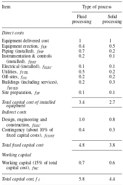
2.1 The Role of Process Economics 17 2.2 Capital Cost for New Design 17 2.3 Capital Cost for Retrofit 23 2.4 Annualized Capital Cost 24 2.5 Operating Cost 25 2.6 Simple Economic Criteria 28 2.7 Project Cash Flow and Economic
Evaluation 29
2.8 Investment Criteria 30 2.9 Process Economics – Summary 31
2.10 Exercises 32
References 33
Chapter 3 Optimization 35
3.1 Objective Functions 35 3.2 Single-variable Optimization 37 3.3 Multivariable Optimization 38 3.4 Constrained Optimization 42 3.5 Linear Programming 43
3.6 Nonlinear Programming 45 3.7 Profile Optimization 46 3.8 Structural Optimization 48 3.9 Solution of Equations
using Optimization 52 3.10 The Search for Global
Optimality 53
3.11 Summary – Optimization 54
3.12 Exercises 54
References 56
Chapter 4 Thermodynamic Properties and
Phase Equilibrium 57
4.1 Equations of State 57 4.2 Phase Equilibrium for Single
Components 59
4.3 Fugacity and Phase Equilibrium 60 4.4 Vapor–Liquid Equilibrium 60 4.5 Vapor–Liquid Equilibrium Based on
Activity Coefficient Models 62 4.6 Vapor–Liquid Equilibrium Based on
Equations of State 64 4.7 Calculation of Vapor–Liquid
Equilibrium 64
4.8 Liquid–Liquid Equilibrium 70 4.9 Liquid–Liquid Equilibrium Activity
Coefficient Models 71 4.10 Calculation of Liquid–Liquid
Equilibrium 71
4.11 Calculation of Enthalpy 72 4.12 Calculation of Entropy 74 4.13 Phase Equilibrium and Thermodynamic
Properties – Summary 74
4.14 Exercises 74
References 76
Chapter 5 Choice of Reactor I – Reactor
Performance 77
5.8 Choice of Reactor
Performance – Summary 94
5.9 Exercises 95
References 96
Chapter 6 Choice of Reactor II - Reactor
Conditions 97
6.1 Reaction Equilibrium 97 6.2 Reactor Temperature 100 6.3 Reactor Pressure 107 6.4 Reactor Phase 108 6.5 Reactor Concentration 109 6.6 Biochemical Reactions 114
6.7 Catalysts 114
6.8 Choice of Reactor
Conditions – Summary 117
6.9 Exercises 118
References 120
Chapter 7 Choice of Reactor III – Reactor
Configuration 121
7.1 Temperature Control 121 7.2 Catalyst Degradation 123 7.3 Gas–Liquid and Liquid–Liquid
Reactors 124
7.4 Reactor Configuration 127 7.5 Reactor Configuration for
Heterogeneous Solid-Catalyzed
Reactions 133
7.6 Reactor Configuration from
Optimization of a Superstructure 133 7.7 Choice of Reactor
Configuration – Summary 139
7.8 Exercises 139
References 140
Chapter 8 Choice of Separator for
Heterogeneous Mixtures 143
8.1 Homogeneous and Heterogeneous
Separation 143
8.2 Settling and Sedimentation 143 8.3 Inertial and Centrifugal Separation 147 8.4 Electrostatic Precipitation 149
8.5 Filtration 150
8.6 Scrubbing 151
8.7 Flotation 152
8.8 Drying 153
8.9 Separation of Heterogeneous
Mixtures – Summary 154
8.10 Exercises 154
References 155
Chapter 9 Choice of Separator for Homogeneous Fluid Mixtures
I – Distillation 157
9.1 Single-Stage Separation 157 9.2 Distillation 157 9.3 Binary Distillation 160 9.4 Total and Minimum Reflux
Conditions for Multicomponent
Mixtures 163
9.5 Finite Reflux Conditions for
Multicomponent Mixtures 170 9.6 Choice of Operating Conditions 175 9.7 Limitations of Distillation 176 9.8 Separation of Homogeneous Fluid
Mixtures by Distillation – Summary 177
9.9 Exercises 178
References 179
Chapter 10 Choice of Separator for Homogeneous Fluid Mixtures
II – Other Methods 181
10.1 Absorption and Stripping 181 10.2 Liquid–Liquid Extraction 184 10.3 Adsorption 189
10.4 Membranes 193
10.5 Crystallization 203 10.6 Evaporation 206 10.7 Separation of Homogeneous Fluid
Mixtures by Other
Methods – Summary 208
10.8 Exercises 209
References 209
Chapter 11 Distillation Sequencing 211
11.1 Distillation Sequencing Using
Simple Columns 211 11.2 Practical Constraints Restricting
Options 211
11.3 Choice of Sequence for Simple
Nonintegrated Distillation Columns 212 11.4 Distillation Sequencing Using
Columns With More Than Two
Products 217
11.5 Distillation Sequencing Using
Thermal Coupling 220 11.6 Retrofit of Distillation Sequences 224 11.7 Crude Oil Distillation 225 11.8 Distillation Sequencing Using
Optimization of a Superstructure 228 11.9 Distillation Sequencing – Summary 230 11.10 Exercises 231
Contents ix
Chapter 12 Distillation Sequencing for
Azeotropic Distillation 235
12.1 Azeotropic Systems 235 12.2 Change in Pressure 235 12.3 Representation of Azeotropic
Distillation 236
12.4 Distillation at Total Reflux
Conditions 238
12.5 Distillation at Minimum Reflux
Conditions 242
12.6 Distillation at Finite Reflux
Conditions 243
12.7 Distillation Sequencing Using an
Entrainer 246
12.8 Heterogeneous Azeotropic
Distillation 251
12.9 Entrainer Selection 253 12.10 Trade-offs in Azeotropic Distillation 255 12.11 Multicomponent Systems 255 12.12 Membrane Separation 255 12.13 Distillation Sequencing for
Azeotropic Distillation – Summary 256 12.14 Exercises 257
References 258
Chapter 13 Reaction, Separation and Recycle
Systems for Continuous Processes 259
13.1 The Function of Process Recycles 259 13.2 Recycles with Purges 264 13.3 Pumping and Compression 267 13.4 Simulation of Recycles 276 13.5 The Process Yield 280 13.6 Optimization of Reactor Conversion 281 13.7 Optimization of Processes Involving
a Purge 283
13.8 Hybrid Reaction and Separation 284 13.9 Feed, Product and Intermediate
Storage 286
13.10 Reaction, Separation and Recycle Systems for Continuous
Processes – Summary 288 13.11 Exercises 289
References 290
Chapter 14 Reaction, Separation and Recycle
Systems for Batch Processes 291
14.1 Batch Processes 291 14.2 Batch Reactors 291 14.3 Batch Separation Processes 297 14.4 Gantt Charts 303 14.5 Production Schedules for Single
Products 304
14.6 Production Schedules for Multiple
Products 305
14.7 Equipment Cleaning and Material
Transfer 306
14.8 Synthesis of Reaction and Separation Systems for Batch
Processes 307
14.9 Optimization of Batch Processes 311 14.10 Storage in Batch Processes 312 14.11 Reaction and Separation Systems for
Batch Processes – Summary 313 14.12 Exercises 313
References 315
Chapter 15 Heat Exchanger Networks
I – Heat Transfer Equipment 317
15.1 Overall Heat Transfer Coefficients 317 15.2 Heat Transfer Coefficients and
Pressure Drops for Shell-and-Tube
Heat Exchangers 319 15.3 Temperature Differences in
Shell-and-Tube Heat Exchangers 324 15.4 Allocation of Fluids in
Shell-and-Tube Heat Exchangers 329 15.5 Extended Surface Tubes 332 15.6 Retrofit of Heat Exchangers 333 15.7 Condensers 337 15.8 Reboilers and Vaporizers 342 15.9 Other Types of Heat Exchange
Equipment 346
15.10 Fired Heaters 348 15.11 Heat Transfer
Equipment – Summary 354 15.12 Exercises 354
References 356
Chapter 16 Heat Exchanger Networks
II – Energy Targets 357
16.1 Composite Curves 357 16.2 The Heat Recovery Pinch 361 16.3 Threshold Problems 364 16.4 The Problem Table Algorithm 365 16.5 Nonglobal Minimum Temperature
Differences 370
16.6 Process Constraints 370 16.7 Utility Selection 372
16.8 Furnaces 374
16.9 Cogeneration (Combined Heat and
Power Generation) 376 16.10 Integration Of Heat Pumps 381 16.11 Heat Exchanger Network Energy
16.12 Exercises 383
References 385
Chapter 17 Heat Exchanger Networks III – Capital and Total Cost
Targets 387
17.1 Number of Heat Exchange Units 387 17.2 Heat Exchange Area Targets 388 17.3 Number-of-shells Target 392 17.4 Capital Cost Targets 393 17.5 Total Cost Targets 395 17.6 Heat Exchanger Network and
Utilities Capital and Total
Costs – Summary 395
17.7 Exercises 396
References 397
Chapter 18 Heat Exchanger Networks
IV – Network Design 399
18.1 The Pinch Design Method 399 18.2 Design for Threshold Problems 404 18.3 Stream Splitting 405 18.4 Design for Multiple Pinches 408 18.5 Remaining Problem Analysis 411 18.6 Network Optimization 413 18.7 The Superstructure Approach to
Heat Exchanger Network Design 416 18.8 Retrofit of Heat Exchanger
Networks 419
18.9 Addition of New Heat Transfer Area
in Retrofit 424
18.10 Heat Exchanger Network
Design – Summary 425 18.11 Exercises 425
References 428
Chapter 19 Heat Exchanger Networks
V – Stream Data 429
19.1 Process Changes for Heat
Integration 429
19.2 The Trade-Offs Between Process Changes, Utility Selection, Energy
Cost and Capital Cost 429 19.3 Data Extraction 430 19.4 Heat Exchanger Network Stream
Data – Summary 437
19.5 Exercises 437
References 438
Chapter 20 Heat Integration of Reactors 439
20.1 The Heat Integration Characteristics
of Reactors 439
20.2 Appropriate Placement of Reactors 441 20.3 Use of the Grand Composite Curve
for Heat Integration of Reactors 442 20.4 Evolving Reactor Design to Improve
Heat Integration 443 20.5 Heat Integration of
Reactors – Summary 444
Reference 444
Chapter 21 Heat Integration of Distillation
Columns 445
21.1 The Heat Integration Characteristics
of Distillation 445 21.2 The Appropriate Placement of
Distillation 445
21.3 Use of the Grand Composite Curve
for Heat Integration of Distillation 446 21.4 Evolving the Design of Simple
Distillation Columns to Improve
Heat Integration 447 21.5 Heat Pumping in Distillation 449 21.6 Capital Cost Considerations 449 21.7 Heat Integration Characteristics of
Distillation Sequences 450 21.8 Heat-integrated Distillation
Sequences Based on the
Optimization of a Superstructure 454 21.9 Heat Integration of Distillation
Columns – Summary 455 21.10 Exercises 456
References 457
Chapter 22 Heat Integration of Evaporators
and Dryers 459
22.1 The Heat Integration Characteristics
of Evaporators 459 22.2 Appropriate Placement of
Evaporators 459
22.3 Evolving Evaporator Design to
Improve Heat Integration 459 22.4 The Heat Integration Characteristics
of Dryers 459
22.5 Evolving Dryer Design to Improve
Heat Integration 460 22.6 Heat Integration of Evaporators and
Contents xi
22.7 Exercises 462
References 463
Chapter 23 Steam Systems and Cogeneration 465
23.1 Boiler Feedwater Treatment 466 23.2 Steam Boilers 468 23.3 Steam Turbines 471 23.4 Gas Turbines 477 23.5 Steam System Configuration 482 23.6 Steam and Power Balances 484 23.7 Site Composite Curves 487 23.8 Cogeneration Targets 490 23.9 Optimization of Steam Levels 493 23.10 Site Power-to-heat Ratio 496 23.11 Optimizing Steam Systems 498 23.12 Steam Costs 502 23.13 Choice of Driver 506 23.14 Steam Systems and
Cogeneration – Summary 507 23.15 Exercises 508
References 510
Chapter 24 Cooling and Refrigeration Systems 513
24.1 Cooling Systems 513 24.2 Recirculating Cooling Water
Systems 513
24.3 Targeting Minimum Cooling Water
Flowrate 516
24.4 Design of Cooling Water Networks 518 24.5 Retrofit of Cooling Water Systems 524 24.6 Refrigeration Cycles 526 24.7 Process Expanders 530 24.8 Choice of Refrigerant for
Compression Refrigeration 532 24.9 Targeting Refrigeration Power for
Compression Refrigeration 535 24.10 Heat Integration of Compression
Refrigeration Processes 539 24.11 Mixed Refrigerants for Compression
Refrigeration 542 24.12 Absorption Refrigeration 544 24.13 Indirect Refrigeration 546 24.14 Cooling Water and Refrigeration
Systems – Summary 546 24.15 Exercises 547
References 549
Chapter 25 Environmental Design for
Atmospheric Emissions 551
25.1 Atmospheric Pollution 551
25.2 Sources of Atmospheric Pollution 552 25.3 Control of Solid Particulate
Emissions to Atmosphere 553 25.4 Control of VOC Emissions to
Atmosphere 554
25.5 Control of Sulfur Emissions 565 25.6 Control of Oxides of Nitrogen
Emissions 569
25.7 Control of Combustion Emissions 573 25.8 Atmospheric Dispersion 574 25.9 Environmental Design for
Atmospheric Emissions – Summary 575 25.10 Exercises 576
References 579
Chapter 26 Water System Design 581
26.1 Aqueous Contamination 583 26.2 Primary Treatment Processes 585 26.3 Biological Treatment Processes 588 26.4 Tertiary Treatment Processes 591
26.5 Water Use 593
26.6 Targeting Maximum Water Reuse
for Single Contaminants 594 26.7 Design for Maximum Water Reuse
for Single Contaminants 596 26.8 Targeting and Design for Maximum
Water Reuse Based on Optimization
of a Superstructure 604 26.9 Process Changes for Reduced Water
Consumption 606
26.10 Targeting Minimum Wastewater Treatment Flowrate for Single
Contaminants 607
26.11 Design for Minimum Wastewater Treatment Flowrate for Single
Contaminants 610
26.12 Regeneration of Wastewater 613 26.13 Targeting and Design for Effluent
Treatment and Regeneration Based
on Optimization of a Superstructure 616 26.14 Data Extraction 617 26.15 Water System Design – Summary 620 26.16 Exercises 620
References 623
Chapter 27 Inherent Safety 625
27.1 Fire 625
27.2 Explosion 626
27.3 Toxic Release 627 27.4 Intensification of Hazardous
27.5 Attenuation of Hazardous Materials 630 27.6 Quantitative Measures of Inherent
Safety 631
27.7 Inherent Safety – Summary 632
27.8 Exercises 632
References 633
Chapter 28 Clean Process Technology 635
28.1 Sources of Waste from Chemical
Production 635
28.2 Clean Process Technology for
Chemical Reactors 636 28.3 Clean Process Technology for
Separation and Recycle Systems 637 28.4 Clean Process Technology for
Process Operations 642 28.5 Clean Process Technology for
Utility Systems 643 28.6 Trading off Clean Process
Technology Options 644 28.7 Life Cycle Analysis 645 28.8 Clean Process Technology –
Summary 646
28.9 Exercises 646
References 647
Chapter 29 Overall Strategy for Chemical
Process Design and Integration 649
29.1 Objectives 649 29.2 The Hierarchy 649 29.3 The Final Design 651
Appendix A Annualization of Capital Cost 653
Appendix B Gas Compression 655
B.1 Reciprocating Compressors 655
B.2 Centrifugal Compressors 658 B.3 Staged Compression 659
Appendix C Heat Transfer Coefficients and Pressure Drop in Shell-and-tube
Heat Exchangers 661
C.1 Pressure Drop and Heat Transfer
Correlations for the Tube-Side 661 C.2 Pressure Drop and Heat Transfer
Correlations for the Shell-Side 662
References 666
Appendix D The Maximum Thermal Effectiveness for 1–2
Shell-and-tube Heat Exchangers 667
Appendix E Expression for the Minimum Number of 1–2 Shell-and-tube
Heat Exchangers for a Given Unit 669
Appendix F Algorithm for the Heat Exchanger
Network Area Target 671
Appendix G Algorithm for the Heat Exchanger
Network Number of Shells Target 673
G.1 Minimum Area Target for Networks
of 1–2 Shells 674
References 677
Appendix H Algorithm for Heat Exchanger
Network Capital Cost Targets 677
Preface
This book deals with the design and integration of chemical processes, emphasizing the conceptual issues that are fundamental to the creation of the process. Chemical process design requires the selection of a series of processing steps and their integration to form a complete manufacturing system. The text emphasizes both the design and selection of the steps as individual operations and their integration to form an efficient process. Also, the process will normally operate as part of an integrated manufacturing site consisting of a number of processes serviced by a common utility system. The design of utility systems has been dealt with so that the interactions between processes and the utility system and the interactions between different processes through the utility system can be exploited to maximize the performance of the site as a whole. Thus, the text integrates equipment, process and utility system design.
Chemical processing should form part of a sustainable industrial activity. For chemical processing, this means that processes should use raw materials as efficiently as is economic and practicable, both to prevent the production of waste that can be environmentally harmful and to preserve the reserves of raw materials as much as possible. Processes should use as little energy as is economic and practicable, both to prevent the buildup of carbon dioxide in the atmosphere from burning fossil fuels and to preserve reserves of fossil fuels. Water must also be consumed in sustainable quantities that do not cause deterioration in the
quality of the water source and the long-term quantity of the reserves. Aqueous and atmospheric emissions must not be environmentally harmful, and solid waste to landfill must be avoided. Finally, all aspects of chemical processing must feature good health and safety practice.
It is important for the designer to understand the limitations of the methods used in chemical process design. The best way to understand the limitations is to understand the derivations of the equations used and the assumptions on which the equations are based. Where practical, the derivation of the design equations has been included in the text.
The book is intended to provide a practical guide to chemical process design and integration for undergraduate and postgraduate students of chemical engineering, practic-ing process designers and chemical engineers and applied chemists working in process development. For undergrad-uate studies, the text assumes basic knowledge of mate-rial and energy balances, fluid mechanics, heat and mass transfer phenomena and thermodynamics, together with basic spreadsheeting skills. Examples have been included throughout the text. Most of these examples do not require specialist software and can be solved using spreadsheet soft-ware. Finally, a number of exercises have been added at the end of each chapter to allow the reader to practice the calculation procedures.
Acknowledgements
The author would like to express gratitude to a number of people who have helped in the preparation and have reviewed parts of the text.
From The University of Manchester: Prof Peter Heggs, Prof Ferda Mavituna, Megan Jobson, Nan Zhang, Constanti-nos Theodoropoulos, Jin-Kuk Kim, Kah Loong Choong, Dhaval Dave, Frank Del Nogal, Ramona Dragomir, Sungwon Hwang, Santosh Jain, Boondarik Leewongtanawit, Guil-ian Liu, Vikas Rastogi, Clemente Rodriguez, Ramagopal Uppaluri, Priti Vanage, Pertar Verbanov, Jiaona Wang, Wen-ling Zhang.
From Alias, UK: David Lott.
From AspenTech: Ian Moore, Eric Petela, Ian Sinclair, Oliver Wahnschafft.
From CANMET, Canada: Alberto Alva-Argaez, Abde-laziz Hammache, Luciana Savulescu, Mikhail Sorin.
From DuPont Taiwan: Janice Kuo.
From Monash University, Australia: David Brennan, Andrew Hoadley.
From UOP, Des Plaines, USA: David Hamm, Greg Maher.
Gratitude is also expressed to Simon Perry, Gareth Maguire, Victoria Woods and Mathew Smith for help in the preparation of the figures.
Nomenclature
a Activity (–), or
constant in cubic equation of state (N·m4·kmol−2), or
correlating coefficient (units depend on application), or
cost law coefficient ($), or order of reaction (–)
A Absorption factor in absorption (–), or annual cash flow ($), or
constant in vapor pressure correlation (N·m−2, bar), or
heat exchanger area (m2) ACF Annual cash flow ($·y−1)
ADCF Annual discounted cash flow ($·y−1) AI Heat transfer area on the inside of tubes
(m2), or
interfacial area (m2, m2·m−3) AM Membrane area (m2)
ANETWORK Heat exchanger network area (m2)
AO Heat transfer area on the outside of
tubes (m2)
ASHELL Heat exchanger area for an individual
shell (m2)
AF Annualization factor for capital cost (–)
b Capital cost law coefficient (units depend on cost law), or
constant in cubic equation of state (m3·kmol−1), or
correlating coefficient (units depend on application), or
order of reaction (–)
bi Bottoms flowrate of Componenti
(kmol·s−1, kmol·h−1) B Bottoms flowrate in distillation
(kmol·s−1, kmol·h−1), or
breadth of device (m), or
constant in vapor pressure correlation (N·K·m−2, bar·K), or
total moles in batch distillation (kmol)
BC Baffle cut for shell-and-tube heat exchangers (–)
BOD Biological oxygen demand (kg·m−3,
mg·l−1)
c Capital cost law coefficient (–), or order of reaction (–)
cD Drag coefficient (–) cF Fanning friction factor (–)
cL Loss coefficient for pipe or pipe fitting (–)
C Concentration (kg·m−3, kmol·m−3,
ppm), or
constant in vapor pressure correlation (K), or
number of components (separate systems) in network design (–)
CB Base capital cost of equipment ($)
Ce Environmental discharge concentration (ppm)
CE Equipment capital cost ($), or
unit cost of energy ($·kW−1, $·MW−1) CF Fixed capital cost of complete
installation ($)
CP Specific heat capacity at constant pressure (kJ·kg−1·K−1,
kJ·kmol−1·K−1)
CP Mean heat capacity at constant pressure
(kJ·kg−1·K−1, kJ·kmol−1·K−1) CV Specific heat capacity at constant
volume (kJ·kg−1·K−1,
kJ·kmol−1·K−1) C∗
Solubility of solute in solvent (kg·kg solvent−1)
CC Cycles of concentration for a cooling tower (–)
COD Chemical oxygen demand (kg·m−3, mg·l−1)
COPHP Coefficient of performance of a heat
pump (–)
COPREF Coefficient of performance of a
CP Capacity parameter in distillation (m·s−1) or
heat capacity flowrate (kW·K−1,
MW·K−1)
CPEX Heat capacity flowrate of heat engine
exhaust (kW·K−1, MW·K−1)
CW Cooling water
d Diameter (µm, m)
di Distillate flowrate of Componenti
(kmol·s−1, kmol·h−1)
dI Inside diameter of pipe or tube (m)
D Distillate flowrate (kmol·s−1, kmol·h−1) DB Tube bundle diameter for shell-and-tube
heat exchangers (m)
DS Shell diameter for shell-and-tube heat
exchangers (m)
DCFRR Discounted cash flowrate of return (%)
E Activation energy of reaction (kJ·kmol−1), or
entrainer flowrate in azeotropic and extractive distillation (kg·s−1,
kmol·s−1), or
extract flowrate in liquid–liquid extraction (kg·s−1, kmol·s−1), or
stage efficiency in separation (–)
EO Overall stage efficiency in distillation and absorption (–)
EP Economic potential ($·y−1)
f Fuel-to-air ratio for gas turbine (–)
fi Capital cost installation factor for
Equipment i (–), or feed flowrate of Componenti
(kmol·s−1, kmol·h−1), or
fugacity of Componenti (N·m−2, bar) fM Capital cost factor to allow for material
of construction (–)
fP Capital cost factor to allow for design pressure (–)
fT Capital cost factor to allow for design
temperature (–)
F Feed flowrate (kg·s−1, kg·h−1,
kmol·s−1, kmol·h−1), or
future worth a sum of money allowing for interest rates ($), or
volumetric flowrate (m3·s−1, m3·h−1) FLV Liquid–vapor flow parameter in
distillation (–)
FT Correction factor for noncountercurrent
flow in shell-and-tube heat exchangers (–)
FTmin Minimum acceptableFT for
noncountercurrent heat exchangers (–)
g Acceleration due to gravity (9.81 m·s−2)
gij Energy of interaction between
Moleculesi andj in the NRTL equation (kJ·kmol−1)
G Free energy (kJ), or
gas flowrate (kg·s−1, kmol·s−1)
Gi Partial molar free energy of Component
i (kJ·kmol−1)
GOi Standard partial molar free energy of Component i(kJ·kmol−1)
h Settling distance of particles (m)
hC Condensing film heat transfer coefficient (W·m−2·K−1,
kW·m−2·K−1)
hI Film heat transfer coefficient for the
inside (W·m−2·K−1, kW·m−2·K−1) hIF Fouling heat transfer coefficient for the
inside (W·m−2·K−1, kW·m−2·K−1) hL Head loss in a pipe or pipe fitting (m)
hNB Nucleate boiling heat transfer
coefficient (W·m−2·K−1,
kW·m−2·K−1)
hO Film heat transfer coefficient for the outside (W·m−2·K−1, kW·m−2·K−1) hOF Fouling heat transfer coefficient for the
outside (W·m−2·K−1, kW·m−2·K−1) hW Heat transfer coefficient for the tube
wall (W·m−2·K−1, kW·m−2·K−1) H Enthalpy (kJ, kJ·kg−1, kJ·kmol−1), or
height (m), or
Henry’s Law Constant (N·m−2, bar,
atm), or
Nomenclature xix
HOi Standard heat of formation of Componenti (kJ·kmol−1) HO Standard heat of reaction (J, kJ) HCOMB Heat of combustion (J·kmol−1,
kJ·kmol−1) HO
COMB Standard heat of combustion at 298 K
(J·kmol−1, kJ·kmol−1)
HP Heat to bring products from standard
temperature to the final temperature (J·kmol−1, kJ·kg−1)
HR Heat to bring reactants from their initial
temperature to standard temperature (J·kmol−1, kJ·kmol−1)
HSTEAM Enthalpy difference between generated
steam and boiler feedwater (kW, MW)
HVAP Latent heat of vaporization (kJ·kg−1,
kJ·kmol−1)
HETP Height equivalent of a theoretical plate (m)
HP High pressure
HR Heat rate for gas turbine (kJ·kWh−1) i Fractional rate of interest on money
(–), or
number of ions (–)
I Total number of hot streams (–)
J Total number of cold streams (–)
k Reaction rate constant (units depend on order of reaction), or
thermal conductivity (W·m−1·K−1,
kW·m−1·K−1)
kG,i Mass transfer coefficient in the gas phase (kmol·m−2·Pa−1·s−1) kij Interaction parameter between
Componentsi andj in an equation of state (–)
kL,i Mass transfer coefficient in the liquid phase (m·s−1)
k0 Frequency factor for heat of reaction (units depend on order of
reaction)
K Overall mass transfer coefficient (kmol·Pa−1·m−2·s−1)or
total number of enthalpy intervals in heat exchanger networks (–)
Ka Equilibrium constant of reaction based on activity (–)
Ki Ratio of vapor to liquid composition at
equilibrium for Componenti (–)
KM,i Equilibrium partition coefficient of
membrane for Componenti (–)
Kp Equilibrium constant of reaction based on partial pressure in the vapor phase (–)
KT Parameter for terminal settling velocity (m·s−1)
Kx Equilibrium constant of reaction based on mole fraction in the liquid phase (–)
Ky Equilibrium constant of reaction based
on mole fraction in vapor phase (–)
L Intercept ratio for turbines (–), or length (m), or
liquid flowrate (kg·s−1, kmol·s−1), or
number of independent loops in a network (–)
LB Distance between baffles in
shell-and-tube heat exchangers (m)
LP Low pressure
m Mass flowrate (kg·s−1), or
molar flowrate (kmol·s−1), or
number of items (–)
M Constant in capital cost correlations (–), or
molar mass (kg·kmol−1)
MP Medium pressure
MCSTEAM Marginal cost of steam ($·t−1)
n Number of items (–), or number of years (–), or polytropic coefficient (–), or slope of Willans’ Line (kJ·kg−1,
MJ·kg−1)
N Number of compression stages (–), or number of moles (kmol), or
number of theoretical stages (–), or rate of transfer of a component
(kmol·s−1·m−3)
Ni Number of moles of Componenti
(kmol)
Ni0 Initial number of moles of Component
i (kmol)
NPT Number of tube passes (–)
NSHELLS Number of number of 1–2 shells in
shell-and-tube heat exchangers (–)
NT Number of tubes (–)
NUNITS Number of units in a heat exchanger
network (–)
NC Number of components in a multicomponent mixture (–)
NPV Net present value ($)
p Partial pressure (N·m−2, bar) pC Pitch configuration factor for tube
layout (–)
pT Tube pitch (m)
P Present worth of a future sum of money ($), or
pressure (N·m−2, bar), or
probability (–), or
thermal effectiveness of 1–2 shell-and-tube heat exchanger (–)
PC Critical pressure (N·m−2, bar)
Pmax Maximum thermal effectiveness of 1–2
shell-and-tube heat exchangers (–)
PM,i Permeability of Componenti for a
membrane (kmol·m·s−1·m−2·bar−1,
kg solvent·m−1·s−1·bar−1) PM,i Permeance of Componenti for a
membrane (m3·m−2·s−1·bar−1) PN−2N Thermal effectiveness overNSHELLS
number of 1–2 shell-and-tube heat exchangers in series (–)
P1−2 Thermal effectiveness over each 1–2
shell-and-tube heat exchanger in series (–)
PSAT Saturated liquid–vapor pressure (N·m−2, bar)
Pr Prandtl number (–)
q Heat flux (W·m−2, kW·m−2), or
thermal condition of the feed in distillation (–), or
Wegstein acceleration parameter for the convergence of recycle calculations (–)
qC Critical heat flux (W·m−2, kW·m−2) qC1 Critical heat flux for a single tube
(W·m−2, kW·m−2)
qi Individual stream heat duty for Stream i (kJ·s−1), or
pure component property measuring the molecular van der Waals surface area for Moleculei in the UNIQUAC Equation (–)
Q Heat duty (kW, MW)
Qc Cooling duty (kW, MW)
Qcmin Target for cold utility (kW, MW)
QCOND Condenser heat duty (kW, MW)
QEVAP Evaporator heat duty (kW, MW)
QEX Heat duty for heat engine exhaust (kW,
MW)
QFEED Heat duty to the feed (kW, MW)
QFUEL Heat from fuel in a furnace, boiler, or
gas turbine (kW, MW)
QH Heating duty (kW, MW)
QHmin Target for hot utility (kW, MW)
QHE Heat engine heat duty (kW, MW)
QHEN Heat exchanger network heat duty (kW,
MW)
QHP Heat pump heat duty (kW, MW)
QLOSS Stack loss from furnace, boiler, or gas
turbine (kW, MW)
QREACT Reactor heating or cooling duty (kW,
MW)
QREB Reboiler heat duty (kW, MW)
QREC Heat recovery (kW, MW)
QSITE Site heating demand (kW, MW)
QSTEAM Heat input for steam generation (kW,
MW)
r Molar ratio (–), or pressure ratio (–), or radius (m)
ri Pure component property measuring the
molecular van der Waals volume for Moleculei in the UNIQUAC Equation (–), or
rate of reaction of Componenti
(kmol−1·s−1), or
recovery of Componenti in separation (–)
Nomenclature xxi
heat capacity ratio of 1–2
shell-and-tube heat exchanger (–), or raffinate flowrate in liquid–liquid
extraction (kg·s−1, kmol·s−1), or ratio of heat capacity flowrates (–), or reflux ratio for distillation (–), or removal ratio in effluent treatment (–),
or
residual error (units depend on application), or
universal gas constant (8314.5 N·m·kmol−1K−1=
J·kmol−1K−1,
8.3145 kJ·kmol−1·K−1) Rmin Minimum reflux ratio (–)
RF Ratio of actual to minimum reflux ratio
(–)
RSITE Site power-to-heat ratio (–) ROI Return on investment (%)
Re Reynolds number (–)
s Reactor space velocity (s−1, min−1,
h−1), or
steam-to-air ratio for gas turbine (–)
S Entropy (kJ·K−1, kJ·kg−1·K−1,
kJ·kmol−1·K−1), or
number of streams in a heat exchanger network (–), or
reactor selectivity (–), or
reboil ratio for distillation (–), or selectivity of a reaction (–), or slack variable in optimization (units
depend on application), or
solvent flowrate (kg·s−1, kmol·s−1), or
stripping factor in absorption (–)
SC Number of cold streams (–) SH Number of hot streams (–) t Time (s, h)
T Temperature (◦
C, K)
TBPT Normal boiling point (◦C, K)
TC Critical temperature (K), or temperature of heat sink (◦
C, K)
TCOND Condenser temperature (◦C, K)
TE Equilibrium temperature (
◦
C, K)
TEVAP Evaporation temperature ( ◦
C, K)
TFEED Feed temperature ( ◦
C, K)
TH Temperature of heat source (
◦
C, K)
TR Reduced temperatureT /TC(–) TREB Reboiler temperature (
◦
C, K)
TS Stream supply temperature (
◦
C)
TSAT Saturation temperature of boiling liquid
(◦
C, K)
TT Stream target temperature (◦
C)
TTFT Theoretical flame temperature (◦C, K)
TW Wall temperature (◦
C)
TWBT Wet bulb temperature (◦C)
T∗
Interval temperature (◦
C)
TLM Logarithmic mean temperature
difference (◦C, K)
Tmin Minimum temperature difference
(◦
C, K)
TSAT Difference in saturation temperature
(◦
C, K)
TTHRESHOLD Threshold temperature difference (
◦
C, K)
TAC Total annual cost ($·y−1)
TOD Total oxygen demand (kg·m−3, mg·l−1) uij Interaction parameter between Molecule
i and Moleculej in the UNIQUAC Equation (kJ·kmol−1)
U Overall heat transfer coefficient (W·m−2·K−1, kW·m−2·K−1) v Velocity (m·s−1)
vT Terminal settling velocity (m·s−1) vV Superficial vapor velocity in empty
column (m·s−1)
V Molar volume (m3·kmol−1), or
vapor flowrate (kg·s−1, kmol·s−1), or
volume (m3), or
volume of gas or vapor adsorbed (m3·kg−1)
Vmin Minimum vapor flow (kg·s−1,
kmol·s−1)
VF Vapor fraction (–)
w Mass of adsorbate per mass of adsorbent (–)
W Shaft power (kW, MW), or shaft work (kJ, MJ)
WGEN Power generated (kW, MW)
WSITE Site power demand (kW, MW)
x Liquid-phase mole fraction (–) or variable in optimization problem (–)
xF Mole fraction in the feed (–)
xD Mole fraction in the distillate (–)
X Reactor conversion (–) or wetness fraction of steam (–)
XE Equilibrium reactor conversion (–)
XOPT Optimal reactor conversion (–)
XP Fraction of maximum thermal
effectivenessPmax allowed in a 1–2
shell-and-tube heat exchanger (–)
XP Cross-pinch heat transfer in heat exchanger network (kW, MW)
y Integer variable in optimization (–), or vapor-phase mole fraction (–)
z Elevation (m), or feed mole fraction (–)
Z Compressibility of a fluid (–)
GREEK LETTERS
α Constant in cubic equation of state (–), or
constants in vapor pressure correlation (units depend on which constant), or fraction open of a valve (–)
αij Ideal separation factor or selectivity of
membrane between Components i
and j (–), or
parameter characterizing the tendency of Moleculei and Moleculej to be distributed in a random fashion in the NRTL equation (–), or
relative volatility between Components
i andj (–)
αLH Relative volatility between light and
heavy key components (–)
βij Separation factor between Components
i andj (–)
γ Ratio of heat capacities for gases and vapors (–)
γi Activity coefficient for Componenti
(–)
δM Membrane thickness (m)
ε Extraction factor in liquid–liquid extraction (–), or
pipe roughness (mm)
η Carnot factor (–), or efficiency (–)
ηBOILER Boiler efficiency (–)
ηCOGEN Cogeneration efficiency (–)
ηGT Efficiency of gas turbine (–)
ηIS Isentropic efficiency of compression or
expansion (–)
ηMECH Mechanical efficiency of steam turbine
(–)
ηP Polytropic efficiency of compression or
expansion (–)
ηPOWER Power generation efficiency (–)
ηST Efficiency of steam turbine (–)
θ Fraction of feed permeated through membrane (–), or
root of the Underwood Equation (–)
λ Ratio of latent heats of vaporization (–)
λij Energy parameter characterizing the
interaction of Moleculei with Moleculej (kJ·kmol−1) µ Fluid viscosity (kg·m−1·s−1,
mN·s·m−2=cP)
π Osmotic pressure (N·m−2, bar) ρ Density (kg·m−3, kmol·m−3) σ Surface tension
(mN·m−1=mJ·m−2=dyne·cm−1) τ Reactor space time (s, min, h) or
residence time (s, min, h)
φ Cost-weighing factor applied to film heat transfer coefficients to allow for mixed materials of construction, pressure rating, and equipment types in heat exchanger networks (–), or fugacity coefficient (–)
ω Acentric factor (–)
SUBSCRIPTS
B Blowdown, or bottoms in distillation
Nomenclature xxiii
cont Contribution
C Cold stream, or contaminant
CN Condensing
COND Condensing conditions
CP Continuous phase
CW Cooling water
D Distillate in distillation
DS De-superheating
e Enhanced, or
end zone on the shell-side of a heat exchanger, or
environment
E Extract in liquid–liquid extraction
EVAP Evaporator conditions
EX Exhaust
final Final conditions in a batch
F Feed, or fluid
G Gas phase
H Hot stream
HP Heat pump, or high pressure
i Component number, or stream number
I Inside
IS Isentropic
in Inlet
j Component number, or stream number
k Enthalpy interval number in heat exchanger networks
L Liquid phase
LP Low pressure
m Stage number in distillation and absorption
max Maximum
min Minimum
M Makeup
MIX Mixture
n Stage number in distillation and absorption
out Outlet
O Outside, or
standard conditions
p Stage number in distillation and absorption
prod Products of reaction
P Particle, or permeate
react Reactants
R Raffinate in liquid–liquid extraction
REACT Reaction
S Solvent in liquid–liquid extraction
SAT Saturated conditions
SF Supplementary firing
SUP Superheated conditions
T Treatment
TW Treated water
V Vapor
w Window section on the shell-side of a heat exchanger
W Conditions at the tube wall, or water
∞ Conditions at distillate pinch point
SUPERSCRIPTS
I PhaseI
II PhaseII III PhaseIII
L Liquid
O Standard conditions
V Vapor
1
The Nature of Chemical Process Design and Integration
1.1
CHEMICAL PRODUCTS
Chemical products are essential to modern living standards. Almost all aspects of everyday life are supported by chemical products in one way or another. Yet, society tends to take these products for granted, even though a high quality of life fundamentally depends on them.
When considering the design of processes for the manufacture of chemical products, the market into which they are being sold fundamentally influences the objectives and priorities in the design. Chemical products can be divided into three broad classes:
1. Commodity or bulk chemicals: These are produced in large volumes and purchased on the basis of chemical composition, purity and price. Examples are sulfuric acid, nitrogen, oxygen, ethylene and chlorine.
2. Fine chemicals: These are produced in small volumes and purchased on the basis of chemical composition, purity and price. Examples are chloropropylene oxide (used for the manufacture of epoxy resins, ion-exchange resins and other products), dimethyl formamide (used, for example, as a solvent, reaction medium and interme-diate in the manufacture of pharmaceuticals), n-butyric acid (used in beverages, flavorings, fragrances and other products) and barium titanate powder (used for the man-ufacture of electronic capacitors).
3. Specialty or effect or functional chemicals: These are purchased because of their effect (or function), rather than their chemical composition. Examples are pharma-ceuticals, pesticides, dyestuffs, perfumes and flavorings.
Because commodity and fine chemicals tend to be pur-chased on the basis of their chemical composition alone, they areundifferentiated. For example, there is nothing to choose between 99.9% benzene made by one manufacturer and that made by another manufacturer, other than price and delivery issues. On the other hand, specialty chemicals tend to be purchased on the basis of their effect or function and are therefore differentiated. For example, competitive pharmaceutical products are differentiated according to the efficacy of the product, rather than chemical composition. An adhesive is purchased on the basis of its ability to stick things together, rather than its chemical composition and so on.
Chemical Process Design and Integration R. Smith
2005 John Wiley & Sons, Ltd ISBNs: 0-471-48680-9 (HB); 0-471-48681-7 (PB)
However, undifferentiated and differentiated should be thought of as relative terms rather than absolute terms for chemical products. In practice, chemicals do not tend to be completely undifferentiated or completely differentiated. Commodity and fine chemical products might have impurity specifications as well as purity specifications. Traces of impurities can, in some cases, give some differentiation between different manufacturers of commodity and fine chemicals. For example, 99.9% acrylic acid might be considered to be an undifferentiated product. However, traces of impurities, at concentrations of a few parts per million, can interfere with some of the reactions in which it is used and can have important implications for some of its uses. Such impurities might differ between different manufacturing processes. Not all specialty products are differentiated. For example, pharmaceutical products like aspirin (acetylsalicylic acid) are undifferentiated. Different manufacturers can produce aspirin and there is nothing to choose between these products, other than the price and differentiation created through marketing of the product.
Scale of production also differs between the three classes of chemical products. Fine and specialty chemicals tend to be produced in volumes less than 1000 t·y−1. On the
other hand, commodity chemicals tend to be produced in much larger volumes than this. However, the distinction is again not so clear. Polymers are differentiated products because they are purchased on the basis of their mechanical properties, but can be produced in quantities significantly higher than 1000 t·y−1.
When a new chemical product is first developed, it can often be protected by a patent in the early years of commercial exploitation. For a product to be eligible to be patented, it must be novel, useful and unobvious. If patent protection can be obtained, this effectively gives the producer a monopoly for commercial exploitation of the product until the patent expires. Patent protection lasts for 20 years from the filing date of the patent. Once the patent expires, competitors can join in and manufacture the product. If competitors cannot wait until the patent expires, then alternative competing products must be developed.
the product depend on both the chemical composition and the method of manufacture.
Figure 1.1 illustrates different productlife cycles1,2. The general trend is that when a new product is introduced into the market, the sales grow slowly until the market is established and then more rapidly once the market is established. If there is patent protection, then competitors will not be able to exploit the same product commercially until the patent expires, when competitors can produce the same product and take market share. It is expected that competitive products will cause sales to diminish later in the product life cycle until sales become so low that a company would be expected to withdraw from the market. In Figure 1.1, ProductAappears to be a poor product that has a short life with low sales volume. It might be that it cannot compete well with other competitive products, and alternative products quickly force the company out of that business. However, a low sales volume is not the main criterion to withdraw from the market. It might be that a product with low volume finds a market niche and can be sold for a high value. On the other hand, if it were competing with other products with similar functions in the same market sector, which keeps both the sale price and volume low, then it would seem wise to withdraw from the market. Product B in Figure 1.1 appears to be a better product, showing a longer life cycle and higher sales volume. This has patent protection but sales decrease rapidly after patent protection is lost, leading to loss of market through competition. Product C in Figure 1.1 is a still better product. This shows high sales volume with the life of the product extended through reformulation of the product1. Finally, Product D in Figure 1.1 shows a
product life cycle that is typical of commodity chemicals. Commodity chemicals tend not to exhibit the same kind of life cycles as fine and specialty chemicals. In the early years of the commercial exploitation, the sales volume grows rapidly to a high volume, but then does not decline and enters a mature period of slow growth, or, in some exceptional cases, slow decline. This is because commodity chemicals tend to have a diverse range of uses. Even though competition might take away some end uses, new end uses are introduced, leading to an extended life cycle.
The different classes of chemical products will have very different added value (the difference between the selling price of the product and the purchase cost of raw materials). Commodity chemicals tend to have low added value, whereas fine and specialty chemicals tend to have high added value. Commodity chemicals tend to be produced in large volumes with low added value, while fine and specialty chemicals tend to be produced in small volumes with high added value.
Because of this, when designing a process for a commodity chemical, it is usually important to keep operating costs as low as possible. The capital cost of the process will tend to be high relative to a process for fine or specialty chemicals because of the scale of production.
When designing a process for specialty chemicals, priority tends to be given to the product, rather than to the process. This is because the unique function of the product must be protected. The process is likely to be small scale and operating costs tend to be less important than with commodity chemical processes. The capital cost of the process will be low relative to commodity chemical processes because of the scale. The time to
Product Sales (t• y−1)
Product D
Product C
Product B
Product A
Patent Expiry Product Reformulation
Time (y)
Formulation of the Design Problem 3
market the product is also likely to be important with specialty chemicals, especially if there is patent protection. If this is the case, then anything that shortens the time from basic research, through product testing, pilot plant studies, process design, construction of the plant to product manufacture will have an important influence on the overall project profitability.
All this means that the priorities in process design are likely to differ significantly, depending on whether a pro-cess is being designed for the manufacture of a commodity, fine or specialty chemical. In commodity chemicals, there is likely to be relatively little product innovation, but intensive process innovation. Also, equipment will be designed for a specific process step. On the other hand, the manufacture of fine and specialty chemicals might involve:
• selling into a market with low volume,
• short product life cycle,
• a demand for a short time to market, and therefore, less time is available for process development, with product and process development proceeding simultaneously.
Because of this, the manufacture of fine and specialty chemicals is often carried out in multipurpose equipment, perhaps with different chemicals being manufactured in the same equipment at different times during the year. The life of the equipment might greatly exceed the life of the product.
The development of pharmaceutical products is such that high-quality products must be manufactured during the development of the process to allow safety and clinical studies to be carried out before full-scale production. Pharmaceutical production represents an extreme case of process design in which the regulatory framework controlling production makes it difficult to make process changes, even during the development stage. Even if significant improvements to processes for pharmaceuticals can be suggested, it might not be feasible to implement them, as such changes might prevent or delay the process from being licensed for production.
1.2
FORMULATION OF THE DESIGN
PROBLEM
Before a process design can be started, the design prob-lem must be formulated. Formulation of the design probprob-lem requires a product specification. If a well-defined chemical product is to be manufactured, then the specification of the product might appear straightforward (e.g. a purify specifica-tion). However, if a specialty product is to be manufactured, it is the functional properties that are important, rather than the chemical properties, and this might require a product designstage in order to specify the product3. The initial
state-ment of the design problem is often ill defined. For example, the design team could be asked to expand the production
capacity of an existing plant that produces a chemical that is a precursor to a polymer product, which is also produced by the company. This results from an increase in the demand for the polymer product and the plant producing the precur-sor currently being operated at its maximum capacity. The designer might well be given a specification for the expan-sion. For example, the marketing department might assess that the market could be expanded by 30% over a two-year period, which would justify a 30% expansion in the process for the precursor. However, the 30% projection can easily be wrong. The economic environment can change, leading to the projected increase being either too large or too small. It might also be possible to sell the polymer precursor in the market to other manufacturers of the polymer and justify an expansion even larger than 30%. If the polymer precursor can be sold in the marketplace, is the current purity specification of the company suitable for the marketplace? Perhaps the marketplace demands a higher purity than what is currently the company specification. Perhaps the current specification is acceptable, but if the specification could be improved, the product could be sold for a higher value and/or at a greater volume. An option might be to not expand the production of the polymer precursor to 30%, but instead to purchase it from the market. If it is purchased from the market, is it likely to be up to the company specifications, or will it need some purification before it is suitable for the company’s polymer process? How reliable will the market source be? All these uncertainties are related more to market supply and demand issues than to specific process design issues.
Closer examination of the current process design might lead to the conclusion that the capacity can be expanded by 10% with a very modest capital investment. A further increase to 20% would require a significant capital investment, but an expansion to 30% would require an extremely large capital investment. This opens up further options. Should the plant be expanded by 10% and a market source identified for the balance? Should the plant be expanded to 20% similarly? If a real expansion in the market place is anticipated and expansion to 30% would be very expensive, why not be more aggressive and instead of expanding the existing process, build an entirely new process? If a new process is to be built, then what should be the process technology? New process technology might have been developed since the original plant was built that enables the same product to be manufactured at a much lower cost. If a new process is to be built, where should it be built? It might make more sense to build it in another country that would allow lower operating costs, and the product could be shipped back to be fed to the existing polymer process. At the same time, this might stimulate the development of new markets in other countries, in which case, what should be the capacity of the new plant?
ill-defined problem, the design team must create a series of very specific options and these should then be compared on the basis of a common set of assumptions regarding, for example, raw materials prices and product prices. Having specified an option, this gives the design team a well-defined problem to which the methods of engineering and economic analysis can be applied.
In examining a design option, the design team should start out by examining the problem at the highest level, in terms of its feasibility with the minimum of detail to ensure the design option is worth progressing4. Is there a
large difference between the value of the product and the cost of the raw materials? If the overall feasibility looks attractive, then more detail can be added, the option re-evaluated, further detail added, and so on. Byproducts might play a particularly important role in the economics. It might be that the current process produces some byproducts that can be sold in small quantities to the market. But, as the process is expanded, there might be market constraints for the new scale of production. If the byproducts cannot be sold, how does this affect the economics?
If the design option appears to be technically and eco-nomically feasible, then additional detail can be considered. Material and energy balances can be formulated to give a better definition to the inner workings of the process and a more detailed process design can be developed. The design calculations for this will normally be solved to a high level of precision. However, a high level of preci-sion cannot usually be justified in terms of the operation of the plant after it has been built. The plant will almost never work precisely at its original design flowrates, temperatures, pressures and compositions. This might be because the raw materials are slightly different than what is assumed in the design. The physical properties assumed in the calculations might have been erroneous in some way, or operation at the original design conditions might create corrosion or foul-ing problems, or perhaps the plant cannot be controlled adequately at the original conditions, and so on, for a mul-titude of other possible reasons. The instrumentation on the plant will not be able to measure the flowrates, tem-peratures, pressures and compositions as accurately as the calculations performed. High precision might be required for certain specific parts of the design. For example, the polymer precursor might need certain impurities to be very tightly controlled, perhaps down to the level of parts per million. It might be that some contaminant in a waste stream might be exceptionally environmentally harmful and must be extremely well defined in the design calculations.
Even though a high level of precision cannot be justified in many cases in terms of the plant operation, the design calculations will normally be carried out to a reasonably high level of precision. The value of precision in design calculations is that the consistency of the calculations can be checked to allow errors or poor assumptions to be identified.
It also allows the design options to be compared on a valid like-for-like basis.
Because of all the uncertainties in carrying out a design, the specifications are often increased beyond those indicated by the design calculations and the plant is overdesigned, or contingency is added, through the application of safety factors to the design. For example, the designer might calculate the number of distillation plates required for a distillation separation using elaborate calculations to a high degree of precision, only to add an arbitrary extra 10% to the number of plates for contingency. This allows for the feed to the unit not being exactly as specified, errors in the physical properties, upset conditions in the plant, control requirements, and so on. If too little contingency is added, the plant might not work. If too much contingency is added, the plant will not only be unnecessarily expensive, but too much overdesign might make the plant difficult to operate and might lead to a less efficient plant. For example, the designer might calculate the size of a heat exchanger and then add in a large contingency and significantly oversize the heat exchanger. The lower fluid velocities encountered by the oversized heat exchanger can cause it to have a poorer performance and to foul up more readily than a smaller heat exchanger. Thus, a balance must be made between different risks.
In summary, the original problem posed to process design teams is often ill-defined, even though it might appear to be well defined in the original design specification. The design team must then formulate a series of plausible design options to be screened by the methods of engineering and economic analysis. These design options are formulated into very specific design problems. Some design options might be eliminated early by high-level arguments or simple calculations. Others will require more detailed examination. In this way, the design team turns the ill-defined problem into a well-defined one for analysis. To allow for the many unquantifiable uncertainties, overdesign is used. Too little overdesign might lead to the plant not working. Too much overdesign will lead to the plant becoming unnecessarily expensive, and perhaps difficult to operate and less efficient. A balance must be made between different risks.
Consider the basic features of the design of chemical processes now.
1.3
CHEMICAL PROCESS DESIGN
AND INTEGRATION
The Hierarchy of Chemical Process Design and Integration 5
Feed Streams
Feed Streams
Product Streams
Product Streams (a) Process design starts with the synthesis of a process to convert raw
materials into desired products.
(b) Simulation predicts how a process would behave if it was constructed.
d. ?
Figure 1.2 Synthesis is the creation of a process to transform feed streams into product streams. Simulation predicts how it would behave if it was constructed.
overall transformation (Figure 1.2a). Thus, thesynthesis of a chemical process involves two broad activities. First, vidual transformation steps are selected. Second, these indi-vidual transformations are interconnected to form a complete process that achieves the required overall transformation. A
flowsheet is a diagrammatic representation of the process steps with their interconnections.
Once the flowsheet structure has been defined, a
simulation of the process can be carried out. A simulation is a mathematical model of the process that attempts to predict how the process would behave if it were constructed (Figure 1.2b). Having created a model of the process, the flowrates, compositions, temperatures and pressures of the feeds can be assumed. The simulation model then predicts the flowrates, compositions, temperatures, and pressures of the products. It also allows the individual items of equipment in the process to be sized and predicts, for example, how much raw material is being used or how much energy is being consumed. The performance of the design can then be evaluated. There are many facets to the evaluation of performance. Good economic performance is an obvious first criterion, but it is certainly not the only one. Chemical processes should be designed as part of a sustainable industrial activity that retains the capacity of ecosystems to support both life and industrial activity into the future. Sustainable industrial activity must meet the needs of the present, without compromising the needs of future generations. For chemical process design, this means that processes should use raw materials as efficiently as is economic and practicable, both to prevent the production of waste that can be environmentally harmful and to preserve the reserves of raw materials as much as possible. Processes should use as little energy as is economic and practicable, both to prevent the build-up of carbon dioxide in the atmosphere from burning fossil fuels and to preserve the reserves of fossil fuels. Water must also be consumed in
sustainable quantities that do not cause deterioration in the quality of the water source and the long-term quantity of the reserves. Aqueous and atmospheric emissions must not be environmentally harmful, and solid waste to landfill must be avoided.
The process must also meet required health and safety criteria. Start-up, emergency shutdown and ease of control are other important factors. Flexibility, that is, the ability to operate under different conditions, such as differences in feedstock and product specification, may be important. Availability, that is, the number of operating hours per year, may also be critically important. Uncertainty in the design, for example, resulting from poor design data, or uncertainty in the economic data, might guide the design away from certain options. Some of these factors, such as economic performance, can be readily quantified; others, such as safety, often cannot. Evaluation of the factors that are not readily quantifiable, the intangibles, requires the judgment of the design team.
Once the basic performance of the design has been eval-uated, changes can be made to improve the performance; the process isoptimized. These changes might involve the synthesis of alternative structures, that is, structural opti-mization. Thus, the process is simulated and evaluated again, and so on, optimizing the structure. Alternatively, each structure can be subjected to parameter optimization
by changing operating conditions within that structure.
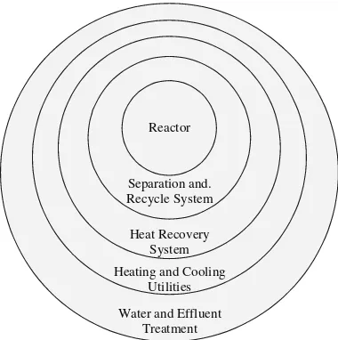
1.4
THE HIERARCHY OF CHEMICAL
PROCESS DESIGN AND
INTEGRATION
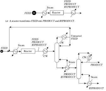
Consider the process illustrated in Figure 1.35. The process
requires a reactor to transform the FEED intoPRODUCT
(Figure 1.3a). Unfortunately, not all theFEED reacts. Also, part of theFEED reacts to form BYPRODUCT instead of the desired PRODUCT. A separation system is needed to isolate the PRODUCT at the required purity. Figure 1.3b shows one possible separation system consisting of two distillation columns. The unreacted FEED in Figure 1.3b is recycled, and the PRODUCT and BYPRODUCT are removed from the process. Figure 1.3b shows a flowsheet where all heating and cooling is provided by external
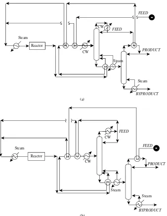
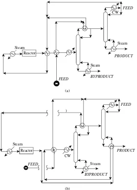
utilities (steam and cooling water in this case). This flowsheet is probably too inefficient in its use of energy, and heat would be recovered. Thus, heat integration is carried out to exchange heat between those streams that need to be cooled and those that need to be heated. Figure 1.45 shows
two possible designs for the heat exchanger network, but many other heat integration arrangements are possible.
BYPRODUCT Steam
FEED
FEED PRODUCT BYPRODUCT
CW
Steam Reactor
CW
CW
Steam PRODUCT
BYPRODUCT
(b) To isolate the PRODUCT and recycle unreacted FEED a separation system is needed. (a) A reactor transforms FEED into PRODUCT and BYPRODUCT.
Unreacted FEED
PRODUCT Steam
FEED
FEED PRODUCT BYPRODUCT
[image:32.612.145.482.76.368.2]Reactor
Figure 1.3 Process design starts with the reactor. The reactor design di