Applied Numerical Methods
with MATLAB
®for Engineers and Scientists
Third Edition
Steven C. Chapra
Berger Chair in Computing and Engineering Tufts UniversityAPPLIED NUMERICAL METHODS WITH MATLAB FOR ENGINEERS AND SCIENTISTS, THIRD EDITION Published by McGraw-Hill, a business unit of The McGraw-Hill Companies, Inc., 1221 Avenue of the Americas, New York, NY 10020. Copyright © 2012 by The McGraw-Hill Companies, Inc. All rights reserved. Previous editions © 2008 and 2005. No part of this publication may be reproduced or distributed in any form or by any means, or stored in a database or retrieval system, without the prior written consent of The McGraw-Hill Companies, Inc., including, but not limited to, in any network or other electronic storage or transmission, or broadcast for distance learning.
Some ancillaries, including electronic and print components, may not be available to customers outside the United States. This book is printed on acid-free paper.
1 2 3 4 5 6 7 8 9 0 DOC/DOC 1 0 9 8 7 6 5 4 3 2 1 ISBN 978-0-07-340110-2
MHID 0-07-340110-2
Vice President & Editor-in-Chief: Marty Lange Vice President EDP/Central Publishing Services:
Kimberly Meriwether David Publisher: Raghothaman Srinivasan Sponsoring Editor: Peter E. Massar Marketing Manager: Curt Reynolds Development Editor: Lorraine Buczek Project Manager: Melissa M. Leick
Design Coordinator: Brenda A. Rolwes
Cover Design: Studio Montage, St. Louis, Missouri Cover Credit: ©Brand X/Jupiter Images RF Buyer: Kara Kudronowicz
Media Project Manager: Balaji Sundararaman Compositor:MPS Limited, a Macmillan Company Typeface: 10/12 Times
Printer: R.R. Donnelley
All credits appearing on page or at the end of the book are considered to be an extension of the copyright page.
MATLAB and Simulink are registered trademarks of The MathWorks, Inc. See www.mathworks.com/trademarks for a list of additional trademarks. The MathWorks Publisher Logo identifies books that contain “MATLAB®” content. Used with permission.
The MathWorks does not warrant the accuracy of the text or exercises in this book. This book’s use or discussion “MATLAB®”
software or related products does not constitute endorsement or sponsorship by The MathWorks of a particular use of the “MATLAB®” software or related products.
For MATLAB®and Simulink product information, or information on other related products, please contact:
The MathWorks, Inc. 3 Apple Hill Drive
Natick, MA, 01760-2098 USA Tel: 508-647-7000
Fax: 508-647-7001
E-mail: [email protected] Web: www.mathworks.com
Library of Congress Cataloging-in-Publication Data Chapra, Steven C.
Applied numerical methods with MATLAB for engineers and scientists / Steven C. Chapra. — 3rd ed. p. cm.
ISBN 978-0-07-340110-2 (alk. paper)
1. Numerical analysis—Data processing—Textbooks. 2. MATLAB—Textbooks. I. Title. QA297.C4185 2012
To
My brothers,
ABOUT THE AUTHOR
Steve Chapra teaches in the Civil and Environmental Engineering Department at Tufts University, where he holds the Louis Berger Chair in Computing and Engineering. His other books include Numerical Methods for Engineers andSurface Water-Quality Modeling.
Steve received engineering degrees from Manhattan College and the University of Michigan. Before joining the faculty at Tufts, he worked for the Environmental Protection Agency and the National Oceanic and Atmospheric Administration, and taught at Texas A&M University and the University of Colorado. His general research interests focus on surface water-quality modeling and advanced computer applications in environmental engineering.
He has received a number of awards for his scholarly contributions, including the Rudolph Hering Medal, the Meriam / Wiley Distinguished Author Award, and the Chandler-Misener Award. He has also been recognized as the outstanding teacher among the engi-neering faculties at both Texas A&M University (1986 Tenneco Award) and the University of Colorado (1992 Hutchinson Award).
Steve was originally drawn to environmental engineering and science because of his love of the outdoors. He is an avid fly fisherman and hiker. An unapologetic nerd, his love affair with computing began when he was first introduced to Fortran programming as an undergraduate in 1966. Today, he feels truly blessed to be able to meld his love of mathe-matics, science, and computing with his passion for the natural environment. In addition, he gets the bonus of sharing it with others through his teaching and writing!
Beyond his professional interests, he enjoys art, music (especially classical music, jazz, and bluegrass), and reading history. Despite unfounded rumors to the contrary, he never has, and never will, voluntarily bungee jump or sky dive.
If you would like to contact Steve, or learn more about him, visit his home page at http://engineering.tufts.edu/cee/people/chapra/ or e-mail him at [email protected].
v
CONTENTS
About the Author iv
Preface xiii
P
ARTO
NEModeling, Computers, and Error Analysis 1
1.1 Motivation 1
1.2 Part Organization 2
CHAPTER 1
Mathematical Modeling, Numerical Methods, and Problem Solving 4
1.1 A Simple Mathematical Model 5
1.2 Conservation Laws in Engineering and Science 12 1.3 Numerical Methods Covered in This Book 13 1.4 Case Study: It’s a Real Drag 17
Problems 20
CHAPTER 2
MATLAB Fundamentals 24
2.1 The MATLAB Environment 25 2.2 Assignment 26
2.3 Mathematical Operations 32 2.4 Use of Built-In Functions 35 2.5 Graphics 38
2.6 Other Resources 40
2.7 Case Study: Exploratory Data Analysis 42 Problems 44
CHAPTER 3
Programming with MATLAB 48
3.3 Structured Programming 57 3.4 Nesting and Indentation 71 3.5 Passing Functions to M-Files 74
3.6 Case Study: Bungee Jumper Velocity 79 Problems 83
CHAPTER 4
Roundoff and Truncation Errors 88
4.1 Errors 89
4.2 Roundoff Errors 95 4.3 Truncation Errors 103 4.4 Total Numerical Error 114
4.5 Blunders, Model Errors, and Data Uncertainty 119 Problems 120
P
ARTT
WORoots and Optimization 123
2.1 Overview 123
2.2 Part Organization 124
CHAPTER 5
Roots: Bracketing Methods 126
5.1 Roots in Engineering and Science 127 5.2 Graphical Methods 128
5.3 Bracketing Methods and Initial Guesses 129 5.4 Bisection 134
5.5 False Position 140
5.6 Case Study: Greenhouse Gases and Rainwater 144 Problems 147
CHAPTER 6
Roots: Open Methods 151
6.1 Simple Fixed-Point Iteration 152 6.2 Newton-Raphson 156
6.3 Secant Methods 161 6.4 Brent’s Method 163
6.5 MATLAB Function: fzero 168 6.6 Polynomials 170
CHAPTER 7
Optimization 182
7.1 Introduction and Background 183 7.2 One-Dimensional Optimization 186 7.3 Multidimensional Optimization 195
7.4 Case Study: Equilibrium and Minimum Potential Energy 197 Problems 199
P
ARTT
HREELinear Systems 205
3.1 Overview 205
3.2 Part Organization 207
CHAPTER 8
Linear Algebraic Equations and Matrices 209
8.1 Matrix Algebra Overview 211
8.2 Solving Linear Algebraic Equations with MATLAB 220 8.3 Case Study: Currents and Voltages in Circuits 222 Problems 226
CHAPTER 9
Gauss Elimination 229
9.1 Solving Small Numbers of Equations 230 9.2 Naive Gauss Elimination 235
9.3 Pivoting 242
9.4 Tridiagonal Systems 245
9.5 Case Study: Model of a Heated Rod 247 Problems 251
CHAPTER 10
LUFactorization 254
10.1 Overview of LUFactorization 255 10.2 Gauss Elimination as LUFactorization 256 10.3 Cholesky Factorization 263
10.4 MATLAB Left Division 266 Problems 267
CHAPTER 11
Matrix Inverse and Condition 268
11.1 The Matrix Inverse 268
11.2 Error Analysis and System Condition 272 11.3 Case Study: Indoor Air Pollution 277 Problems 280
CHAPTER 12
Iterative Methods 284
12.1 Linear Systems: Gauss-Seidel 284 12.2 Nonlinear Systems 291
12.3 Case Study: Chemical Reactions 298 Problems 300
CHAPTER 13
Eigenvalues 303
13.1 Mathematical Background 305 13.2 Physical Background 308 13.3 The Power Method 310 13.4 MATLAB Function: eig 313
13.5 Case Study: Eigenvalues and Earthquakes 314 Problems 317
P
ARTF
OURCurve Fitting 321
4.1 Overview 321
4.2 Part Organization 323
CHAPTER 14
Linear Regression 324
14.1 Statistics Review 326
14.2 Random Numbers and Simulation 331 14.3 Linear Least-Squares Regression 336 14.4 Linearization of Nonlinear Relationships 344 14.5 Computer Applications 348
CHAPTER 15
General Linear Least-Squares and Nonlinear Regression 361
15.1 Polynomial Regression 361 15.2 Multiple Linear Regression 365 15.3 General Linear Least Squares 367
15.4 QR Factorization and the Backslash Operator 370 15.5 Nonlinear Regression 371
15.6 Case Study: Fitting Experimental Data 373 Problems 375
CHAPTER 16
Fourier Analysis 380
16.1 Curve Fitting with Sinusoidal Functions 381 16.2 Continuous Fourier Series 387
16.3 Frequency and Time Domains 390 16.4 Fourier Integral and Transform 391 16.5 Discrete Fourier Transform (DFT) 394 16.6 The Power Spectrum 399
16.7 Case Study: Sunspots 401 Problems 402
CHAPTER 17
Polynomial Interpolation 405
17.1 Introduction to Interpolation 406 17.2 Newton Interpolating Polynomial 409 17.3 Lagrange Interpolating Polynomial 417 17.4 Inverse Interpolation 420
17.5 Extrapolation and Oscillations 421 Problems 425
CHAPTER 18
Splines and Piecewise Interpolation 429
18.1 Introduction to Splines 429 18.2 Linear Splines 431 18.3 Quadratic Splines 435 18.4 Cubic Splines 438
18.5 Piecewise Interpolation in MATLAB 444 18.6 Multidimensional Interpolation 449 18.7 Case Study: Heat Transfer 452 Problems 456
P
ARTF
IVEIntegration and Differentiation 459
5.1 Overview 459
5.2 Part Organization 460
CHAPTER 19
Numerical Integration Formulas 462
19.1 Introduction and Background 463 19.2 Newton-Cotes Formulas 466 19.3 The Trapezoidal Rule 468 19.4 Simpson’s Rules 475
19.5 Higher-Order Newton-Cotes Formulas 481 19.6 Integration with Unequal Segments 482 19.7 Open Methods 486
19.8 Multiple Integrals 486
19.9 Case Study: Computing Work with Numerical Integration 489 Problems 492
CHAPTER 20
Numerical Integration of Functions 497
20.1 Introduction 497 20.2 Romberg Integration 498 20.3 Gauss Quadrature 503 20.4 Adaptive Quadrature 510
20.5 Case Study: Root-Mean-Square Current 514 Problems 517
CHAPTER 21
Numerical Differentiation 521
21.1 Introduction and Background 522
21.2 High-Accuracy Differentiation Formulas 525 21.3 Richardson Extrapolation 528
21.4 Derivatives of Unequally Spaced Data 530 21.5 Derivatives and Integrals for Data with Errors 531 21.6 Partial Derivatives 532
21.7 Numerical Differentiation with MATLAB 533 21.8 Case Study: Visualizing Fields 538
P
ARTS
IXOrdinary Differential Equations 547
6.1 Overview 547
6.2 Part Organization 551
CHAPTER 22
Initial-Value Problems 553
22.1 Overview 555 22.2 Euler’s Method 555
22.3 Improvements of Euler’s Method 561 22.4 Runge-Kutta Methods 567
22.5 Systems of Equations 572
22.6 Case Study: Predator-Prey Models and Chaos 578 Problems 583
CHAPTER 23
Adaptive Methods and Stiff Systems 588
23.1 Adaptive Runge-Kutta Methods 588 23.2 Multistep Methods 597
23.3 Stiffness 601
23.4 MATLAB Application: Bungee Jumper with Cord 607 23.5 Case Study: Pliny’s Intermittent Fountain 608 Problems 613
CHAPTER 24
Boundary-Value Problems 616
24.1 Introduction and Background 617 24.2 The Shooting Method 621 24.3 Finite-Difference Methods 628 Problems 635
APPENDIX A: MATLAB BUILT-IN FUNCTIONS 641
APPENDIX B: MATLAB M-FILE FUNCTIONS 643
BIBLIOGRAPHY 644
INDEX 646
McGraw-Hill Create™
Craft your teaching resources to match the way you teach! With McGraw-Hill Create™, www.mcgrawhillcreate.com, you can easily rearrange chapters, combine material from other content sources, and quickly upload content you have written like your course syllabus or teaching notes. Find the content you need in Create by searching through thou-sands of leading McGraw-Hill textbooks. Arrange your book to fit your teaching style. Create even allows you to personalize your book’s appearance by selecting the cover and adding your name, school, and course information. Order a Create book and you’ll receive a complimentary print review copy in 3–5 business days or a complimentary electronic review copy (eComp) via email in minutes. Go to www.mcgrawhillcreate.com today and register to experience how McGraw-Hill Create™ empowers you to teach your students
yourway.
McGraw-Hill Higher Education and Blackboard Have Teamed Up
Blackboard, the Web-based course-management system, has partnered with McGraw-Hill to better allow students and faculty to use online materials and activities to complement face-to-face teaching. Blackboard features exciting social learning and teaching tools that foster more logical, visually impactful and active learning opportunities for students. You’ll transform your closed-door classrooms into communities where students remain connected to their educational experience 24 hours a day.
This partnership allows you and your students access to McGraw-Hill’s Create™ right from within your Blackboard course—all with one single sign-on. McGraw-Hill and Blackboard can now offer you easy access to industry leading technology and content, whether your campus hosts it, or we do. Be sure to ask your local McGraw-Hill represen-tative for details.
Electronic Textbook Options
PREFACE
This book is designed to support a one-semester course in numerical methods. It has been written for students who want to learn and apply numerical methods in order to solve prob-lems in engineering and science. As such, the methods are motivated by probprob-lems rather than by mathematics. That said, sufficient theory is provided so that students come away with insight into the techniques and their shortcomings.
MATLAB®provides a great environment for such a course. Although other environ-ments (e.g., Excel/VBA, Mathcad) or languages (e.g., Fortran 90, C++) could have been chosen, MATLAB presently offers a nice combination of handy programming fea-tures with powerful built-in numerical capabilities. On the one hand, its M-file program-ming environment allows students to implement moderately complicated algorithms in a structured and coherent fashion. On the other hand, its built-in, numerical capabilities empower students to solve more difficult problems without trying to “reinvent the wheel.”
The basic content, organization, and pedagogy of the second edition are essentially preserved in the third edition. In particular, the conversational writing style is intentionally maintained in order to make the book easier to read. This book tries to speak directly to the reader and is designed in part to be a tool for self-teaching.
That said, this edition differs from the past edition in three major ways: (1) two new chapters, (2) several new sections, and (3) revised homework problems.
1. New Chapters.As shown in Fig. P.1, I have developed two new chapters for this edi-tion. Their inclusion was primarily motivated by my classroom experience. That is, they are included because they work well in the undergraduate numerical methods course I teach at Tufts. The students in that class typically represent all areas of engi-neering and range from sophomores to seniors with the majority at the junior level. In addition, we typically draw a few math and science majors. The two new chapters are: • Eigenvalues. When I first developed this book, I considered that eigenvalues might be deemed an “advanced” topic. I therefore presented the material on this topic at the end of the semester and covered it in the book as an appendix. This sequencing had the ancillary advantage that the subject could be partly motivated by the role of eigenvalues in the solution of linear systems of ODEs. In recent years, I have begun
FIGURE P.1
An outline of this edition. The shaded areas represent new material. In addition, several of the original chapters have been supplemented with new topics.
PART ONE PART TWO PART THREE PART FOUR PART FIVE PART SIX
Modeling, Computers, Roots and Linear Systems Curve Fitting Integration and Ordinary Differential
and Error Analysis Optimization Differentiation Equations
CHAPTER 1 CHAPTER 5 CHAPTER 8 CHAPTER 14 CHAPTER 19 CHAPTER 22 Mathematical Roots: Bracketing Linear Algebraic Linear Regression Numerical Integration Initial-Value Modeling, Numerical Methods Equations Formulas Problems Methods, and Problem and Matrices
Solving
CHAPTER 2 CHAPTER 6 CHAPTER 9 CHAPTER 15 CHAPTER 20 CHAPTER 23 MATLAB Roots: Open Gauss Elimination General Linear Numerical lntegration Adaptive Methods Fundamentals Methods Least-Squares and of Functions and Stiff Systems
Nonlinear Regression
CHAPTER 3 CHAPTER 7 CHAPTER 10 CHAPTER 16 CHAPTER 21 CHAPTER 24 Programming Optimization LUFactorization Fourier Analysis Numerical Boundary-Value
with MATLAB Differentiation Problems
CHAPTER 4 CHAPTER 11 CHAPTER 17 Roundoff and Matrix Inverse Polynomial Truncation Errors and Condition Interpolation
CHAPTER 12 CHAPTER 18 Iterative Methods Splines and Piecewise
Interpolation
PREFACE xv
to move this material up to what I consider to be its more natural mathematical po-sition at the end of the section on linear algebraic equations. By stressing applica-tions (in particular, the use of eigenvalues to study vibraapplica-tions), I have found that students respond very positively to the subject in this position. In addition, it allows me to return to the topic in subsequent chapters which serves to enhance the students’ appreciation of the topic.
• Fourier Analysis. In past years, if time permitted, I also usually presented a lecture at the end of the semester on Fourier analysis. Over the past two years, I have begun presenting this material at its more natural position just after the topic of linear least squares. I motivate the subject matter by using the linear least-squares approach to fit sinusoids to data. Then, by stressing applications (again vibrations), I have found that the students readily absorb the topic and appreciate its value in engineering and science.
It should be noted that both chapters are written in a modular fashion and could be skipped without detriment to the course’s pedagogical arc. Therefore, if you choose, you can either omit them from your course or perhaps move them to the end of the semester. In any event, I would not have included them in the current edition if they did not represent an enhancement within my current experience in the classroom. In particular, based on my teaching evaluations, I find that the stronger, more motivated students actually see these topics as highlights. This is particularly true because MATLAB greatly facilitates their application and inter-pretation.
2. New Content.Beyond the new chapters, I have included new and enhanced sections on a number of topics. The primary additions include sections on animation (Chap. 3), Brent’s method for root location (Chap. 6), LU factorization with pivoting (Chap. 8), ran-dom numbers and Monte Carlo simulation(Chap. 14), adaptive quadrature(Chap. 20), andeventtermination of ODEs (Chap. 23).
3. New Homework Problems.Most of the end-of-chapter problems have been modi-fied, and a variety of new problems have been added. In particular, an effort has been made to include several new problems for each chapter that are more challenging and difficult than the problems in the previous edition.
Aside from the new material and problems, the third edition is very similar to the second. In particular, I have endeavored to maintain most of the features contributing to its pedagog-ical effectiveness including extensive use of worked examples and engineering and scien-tific applications. As with the previous edition, I have made a concerted effort to make this book as “student-friendly” as possible. Thus, I’ve tried to keep my explanations straightfor-ward and practical.
Acknowledgments. Several members of the McGraw-Hill team have contributed to this project. Special thanks are due to Lorraine Buczek, and Bill Stenquist, and Melissa Leick for their encouragement, support, and direction. Ruma Khurana of MPS Limited, a Macmillan Company also did an outstanding job in the book’s final production phase. Last, but not least, Beatrice Sussman once again demonstrated why she is the best copyeditor in the business.
During the course of this project, the folks at The MathWorks, Inc., have truly demon-strated their overall excellence as well as their strong commitment to engineering and science education. In particular, Courtney Esposito and Naomi Fernandes of The Math-Works, Inc., Book Program have been especially helpful.
The generosity of the Berger family, and in particular Fred Berger, has provided me with the opportunity to work on creative projects such as this book dealing with computing and engineering. In addition, my colleagues in the School of Engineering at Tufts, notably Masoud Sanayei, Lew Edgers, Vince Manno, Luis Dorfmann, Rob White, Linda Abriola, and Laurie Baise, have been very supportive and helpful.
Significant suggestions were also given by a number of colleagues. In particular, Dave Clough (University of Colorado–Boulder), and Mike Gustafson (Duke University) pro-vided valuable ideas and suggestions. In addition, a number of reviewers propro-vided useful feedback and advice including Karen Dow Ambtman (University of Alberta), Jalal Behzadi (Shahid Chamran University), Eric Cochran (Iowa State University), Frederic Gibou (Uni-versity of California at Santa Barbara), Jane Grande-Allen (Rice Uni(Uni-versity), Raphael Haftka (University of Florida), Scott Hendricks (Virginia Tech University), Ming Huang (University of San Diego), Oleg Igoshin (Rice University), David Jack (Baylor Univer-sity), Clare McCabe (Vanderbilt UniverUniver-sity), Eckart Meiburg (University of California at Santa Barbara), Luis Ricardez (University of Waterloo), James Rottman (University of California, San Diego), Bingjing Su (University of Cincinnati), Chin-An Tan (Wayne State University), Joseph Tipton (The University of Evansville), Marion W. Vance (Arizona State University), Jonathan Vande Geest (University of Arizona), and Leah J. Walker (Arkansas State University).
It should be stressed that although I received useful advice from the aforementioned individuals, I am responsible for any inaccuracies or mistakes you may find in this book. Please contact me via e-mail if you should detect any errors.
Finally, I want to thank my family, and in particular my wife, Cynthia, for the love, patience, and support they have provided through the time I’ve spent on this project.
Steven C. Chapra Tufts University
PEDAGOGICAL TOOLS
Theory Presented as It Informs Key Concepts. The text is intended for Numerical Meth-ods users, not developers. Therefore, theory is not included for “theory’s sake,” for example no proofs. Theory is included as it informs key concepts such as the Taylor series, convergence, condition, etc. Hence, the student is shown how the theory connects with practical issues in problem solving.
Introductory MATLAB Material. The text includes two introductory chapters on how to use MATLAB. Chapter 2 shows students how to perform computations and create graphs in MATLAB’s standard command mode. Chapter 3 provides a primer on developing numerical programs via MATLAB M-file functions. Thus, the text provides students with the means to develop their own numerical algorithms as well as to tap into MATLAB’s powerful built-in routines.
Algorithms Presented Using MATLAB M-files. Instead of using pseudocode, this book presents algorithms as well-structured MATLAB M-files. Aside from being useful com-puter programs, these provide students with models for their own M-files that they will develop as homework exercises.
Worked Examples and Case Studies. Extensive worked examples are laid out in detail so that students can clearly follow the steps in each numerical computation. The case stud-ies consist of engineering and science applications which are more complex and richer than the worked examples. They are placed at the ends of selected chapters with the intention of (1) illustrating the nuances of the methods, and (2) showing more realistically how the methods along with MATLAB are applied for problem solving.
Problem Sets. The text includes a wide variety of problems. Many are drawn from engi-neering and scientific disciplines. Others are used to illustrate numerical techniques and theoretical concepts. Problems include those that can be solved with a pocket calculator as well as others that require computer solution with MATLAB.
Useful Appendices and Indexes. Appendix A contains MATLAB commands, and Appendix B contains M-file functions.
Textbook Website. A text-specific website is available at www.mhhe.com/chapra. Re-sources include the text images in PowerPoint, M-files, and additional MATLAB reRe-sources.
1 1
P
ART
O
NE
Modeling, Computers,
and Error Analysis
1.1 MOTIVATION
What are numerical methods and why should you study them?
Numerical methodsare techniques by which mathematical problems are formulated so that they can be solved with arithmetic and logical operations. Because digital computers excel at performing such operations, numerical methods are sometimes referred to as com-puter mathematics.
In the pre–computer era, the time and drudgery of implementing such calculations seriously limited their practical use. However, with the advent of fast, inexpensive digital computers, the role of numerical methods in engineering and scientific problem solving has exploded. Because they figure so prominently in much of our work, I believe that nu-merical methods should be a part of every engineer’s and scientist’s basic education. Just as we all must have solid foundations in the other areas of mathematics and science, we should also have a fundamental understanding of numerical methods. In particular, we should have a solid appreciation of both their capabilities and their limitations.
Beyond contributing to your overall education, there are several additional reasons why you should study numerical methods:
1. Numerical methods greatly expand the types of problems you can address. They are capable of handling large systems of equations, nonlinearities, and compli-cated geometries that are not uncommon in engineering and science and that are often impossible to solve analytically with standard calculus. As such, they greatly enhance your problem-solving skills.
your career, you will invariably have occasion to use commercially available prepack-aged computer programs that involve numerical methods. The intelligent use of these programs is greatly enhanced by an understanding of the basic theory underlying the methods. In the absence of such understanding, you will be left to treat such packages as “black boxes” with little critical insight into their inner workings or the validity of the results they produce.
3. Many problems cannot be approached using canned programs. If you are conversant with numerical methods, and are adept at computer programming, you can design your own programs to solve problems without having to buy or commission expensive software.
4. Numerical methods are an efficient vehicle for learning to use computers. Because nu-merical methods are expressly designed for computer implementation, they are ideal for illustrating the computer’s powers and limitations. When you successfully implement numerical methods on a computer, and then apply them to solve otherwise intractable problems, you will be provided with a dramatic demonstration of how computers can serve your professional development. At the same time, you will also learn to acknowl-edge and control the errors of approximation that are part and parcel of large-scale numerical calculations.
5. Numerical methods provide a vehicle for you to reinforce your understanding of math-ematics. Because one function of numerical methods is to reduce higher mathematics to basic arithmetic operations, they get at the “nuts and bolts” of some otherwise obscure topics. Enhanced understanding and insight can result from this alternative perspective.
With these reasons as motivation, we can now set out to understand how numerical methods and digital computers work in tandem to generate reliable solutions to mathemat-ical problems. The remainder of this book is devoted to this task.
1.2 PART ORGANIZATION
This book is divided into six parts. The latter five parts focus on the major areas of numer-ical methods. Although it might be tempting to jump right into this material, Part One con-sists of four chapters dealing with essential background material.
Chapter 1provides a concrete example of how a numerical method can be employed to solve a real problem. To do this, we develop a mathematical model of a free-falling bungee jumper. The model, which is based on Newton’s second law, results in an ordinary differential equation. After first using calculus to develop a closed-form solution, we then show how a comparable solution can be generated with a simple numerical method. We end the chapter with an overview of the major areas of numerical methods that we cover in Parts Two through Six.
Chapters 2 and 3 provide an introduction to the MATLAB®software environment.
Chapter 3shows how MATLAB’s programming modeprovides a vehicle for assem-bling individual commands into algorithms. Thus, our intent is to illustrate how MATLAB serves as a convenient programming environment to develop your own software.
Chapter 4deals with the important topic of error analysis, which must be understood for the effective use of numerical methods. The first part of the chapter focuses on the
roundoff errors that result because digital computers cannot represent some quantities exactly. The latter part addresses truncation errorsthat arise from using an approximation in place of an exact mathematical procedure.
1
Mathematical Modeling,
Numerical Methods,
and Problem Solving
CHAPTER OBJECTIVES
The primary objective of this chapter is to provide you with a concrete idea of what numerical methods are and how they relate to engineering and scientific problem solving. Specific objectives and topics covered are
•
Learning how mathematical models can be formulated on the basis of scientific principles to simulate the behavior of a simple physical system.•
Understanding how numerical methods afford a means to generate solutions in a manner that can be implemented on a digital computer.•
Understanding the different types of conservation laws that lie beneath the models used in the various engineering disciplines and appreciating the difference between steady-state and dynamic solutions of these models.•
Learning about the different types of numerical methods we will cover in this book.4
YOU’VE GOT A PROBLEM
S
uppose that a bungee-jumping company hires you. You’re given the task of predict-ing the velocity of a jumper (Fig. 1.1) as a function of time durpredict-ing the free-fall part of the jump. This information will be used as part of a larger analysis to determine the length and required strength of the bungee cord for jumpers of different mass.of physics and fluid mechanics, you develop the following mathematical model for the rate of change of velocity with respect to time,
dv
dt =g− cd mv
2
where v=downward vertical velocity (m/s), t=time (s), g=the acceleration due to gravity (∼=9.81 m/s2), cd= a lumped drag coefficient (kg/m), and m= the jumper’s
mass (kg). The drag coefficient is called “lumped” because its magnitude depends on fac-tors such as the jumper’s area and the fluid density (see Sec. 1.4).
Because this is a differential equation, you know that calculus might be used to obtain an analytical or exact solution for vas a function of t. However, in the following pages, we will illustrate an alternative solution approach. This will involve developing a computer-oriented numerical or approximate solution.
Aside from showing you how the computer can be used to solve this particular prob-lem, our more general objective will be to illustrate (a) what numerical methods are and (b) how they figure in engineering and scientific problem solving. In so doing, we will also show how mathematical models figure prominently in the way engineers and scientists use numerical methods in their work.
1.1 A SIMPLE MATHEMATICAL MODEL
Amathematical modelcan be broadly defined as a formulation or equation that expresses the essential features of a physical system or process in mathematical terms. In a very gen-eral sense, it can be represented as a functional relationship of the form
Dependent variable = f
independent
variables ,parameters,
forcing functions
(1.1)
where the dependent variableis a characteristic that typically reflects the behavior or state of the system; the independent variables are usually dimensions, such as time and space, along which the system’s behavior is being determined; the parameters are reflective of the system’s properties or composition; and the forcing functions are external influences acting upon it.
The actual mathematical expression of Eq. (1.1) can range from a simple algebraic relationship to large complicated sets of differential equations. For example, on the basis of his observations, Newton formulated his second law of motion, which states that the time rate of change of momentum of a body is equal to the resultant force acting on it. The math-ematical expression, or model, of the second law is the well-known equation
F=ma (1.2)
where Fis the net force acting on the body (N, or kg m/s2), mis the mass of the object (kg), and ais its acceleration (m/s2).
1.1 A SIMPLE MATHEMATICAL MODEL 5
Upward force due to air resistance
Downward force due to gravity
FIGURE 1.1
The second law can be recast in the format of Eq. (1.1) by merely dividing both sides by mto give
a= F
m (1.3)
where ais the dependent variable reflecting the system’s behavior, Fis the forcing func-tion, and mis a parameter. Note that for this simple case there is no independent variable because we are not yet predicting how acceleration varies in time or space.
Equation (1.3) has a number of characteristics that are typical of mathematical models of the physical world.
• It describes a natural process or system in mathematical terms.
• It represents an idealization and simplification of reality. That is, the model ignores neg-ligible details of the natural process and focuses on its essential manifestations. Thus, the second law does not include the effects of relativity that are of minimal importance when applied to objects and forces that interact on or about the earth’s surface at veloc-ities and on scales visible to humans.
• Finally, it yields reproducible results and, consequently, can be used for predictive pur-poses. For example, if the force on an object and its mass are known, Eq. (1.3) can be used to compute acceleration.
Because of its simple algebraic form, the solution of Eq. (1.2) was obtained easily. However, other mathematical models of physical phenomena may be much more complex, and either cannot be solved exactly or require more sophisticated mathematical techniques than simple algebra for their solution. To illustrate a more complex model of this kind, Newton’s second law can be used to determine the terminal velocity of a free-falling body near the earth’s surface. Our falling body will be a bungee jumper (Fig. 1.1). For this case, a model can be derived by expressing the acceleration as the time rate of change of the velocity (dv/dt)and substituting it into Eq. (1.3) to yield
dv
dt = F
m (1.4)
where vis velocity (in meters per second). Thus, the rate of change of the velocity is equal to the net force acting on the body normalized to its mass. If the net force is positive, the object will accelerate. If it is negative, the object will decelerate. If the net force is zero, the object’s velocity will remain at a constant level.
Next, we will express the net force in terms of measurable variables and parameters. For a body falling within the vicinity of the earth, the net force is composed of two oppos-ing forces: the downward pull of gravity FD and the upward force of air resistance FU
(Fig. 1.1):
F=FD+FU (1.5)
If force in the downward direction is assigned a positive sign, the second law can be used to formulate the force due to gravity as
FD=mg (1.6)
Air resistance can be formulated in a variety of ways. Knowledge from the science of fluid mechanics suggests that a good first approximation would be to assume that it is pro-portional to the square of the velocity,
FU = −cdv2 (1.7)
where cdis a proportionality constant called the lumped drag coefficient (kg/m). Thus, the
greater the fall velocity, the greater the upward force due to air resistance. The parameter
cdaccounts for properties of the falling object, such as shape or surface roughness, that
af-fect air resistance. For the present case, cd might be a function of the type of clothing or the
orientation used by the jumper during free fall.
The net force is the difference between the downward and upward force. Therefore, Eqs. (1.4) through (1.7) can be combined to yield
dv
dt =g− cd mv
2 (1.8)
Equation (1.8) is a model that relates the acceleration of a falling object to the forces acting on it. It is a differential equation because it is written in terms of the differential rate of change (dv/dt)of the variable that we are interested in predicting. However, in contrast to the solution of Newton’s second law in Eq. (1.3), the exact solution of Eq. (1.8) for the velocity of the jumper cannot be obtained using simple algebraic manipulation. Rather, more advanced techniques such as those of calculus must be applied to obtain an exact or analytical solution. For example, if the jumper is initially at rest (v=0 at t =0), calculus can be used to solve Eq. (1.8) for
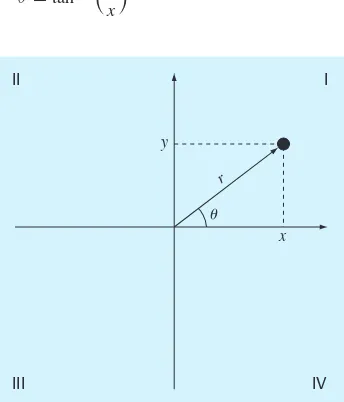
v(t)=
gm
cd tanh
gcd
m t
(1.9)
where tanh is the hyperbolic tangent that can be either computed directly1or via the more elementary exponential function as in
tanhx =e
x−e−x
ex+e−x (1.10)
Note that Eq. (1.9) is cast in the general form of Eq. (1.1) wherev(t)is the dependent variable,tis the independent variable,cdandmare parameters, andgis the forcing function.
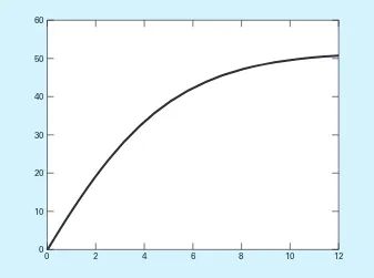
EXAMPLE 1.1 Analytical Solution to the Bungee Jumper Problem
Problem Statement. A bungee jumper with a mass of 68.1 kg leaps from a stationary hot air balloon. Use Eq. (1.9) to compute velocity for the first 12 s of free fall. Also determine the terminal velocity that will be attained for an infinitely long cord (or alternatively, the jumpmaster is having a particularly bad day!). Use a drag coefficient of 0.25 kg/m.
1.1 A SIMPLE MATHEMATICAL MODEL 7
1MATLAB allows direct calculation of the hyperbolic tangent via the built-in function
Solution. Inserting the parameters into Eq. (1.9) yields
v(t)=
9.81(68.1)
0.25 tanh
9.81(0.25)
68.1 t
=51.6938 tanh(0.18977t)
which can be used to compute
t, s v, m/s
0 0
2 18.7292 4 33.1118 6 42.0762 8 46.9575 10 49.4214 12 50.6175 ∞ 51.6938
According to the model, the jumper accelerates rapidly (Fig. 1.2). A velocity of 49.4214 m/s (about 110 mi/hr) is attained after 10 s. Note also that after a sufficiently long
0 20 40 60
0 4 8 12
t, s
Terminal velocity
u
, m/s
FIGURE 1.2
time, a constant velocity, called the terminal velocity, of 51.6983 m/s (115.6 mi/hr) is reached. This velocity is constant because, eventually, the force of gravity will be in bal-ance with the air resistbal-ance. Thus, the net force is zero and acceleration has ceased.
Equation (1.9) is called an analytical or closed-form solution because it exactly satis-fies the original differential equation. Unfortunately, there are many mathematical models that cannot be solved exactly. In many of these cases, the only alternative is to develop a numerical solution that approximates the exact solution.
Numerical methods are those in which the mathematical problem is reformulated so it can be solved by arithmetic operations. This can be illustrated for Eq. (1.8) by realizing that the time rate of change of velocity can be approximated by (Fig. 1.3):
dv
dt
∼
= v
t =
v(ti+1)−v(ti) ti+1−ti
(1.11)
where vand tare differences in velocity and time computed over finite intervals, v(ti)
is velocity at an initial time ti,and v(ti+1)is velocity at some later time ti+1.Note that dv/dt ∼=v/t is approximate because tis finite. Remember from calculus that
dv
dt =tlim→0
v t
Equation (1.11) represents the reverse process.
1.1 A SIMPLE MATHEMATICAL MODEL 9
v(ti⫹1)
ti⫹1 t
⌬t
v(ti)
⌬v
ti True slope
dv/dt
Approximate slope
⌬v v(ti⫹1) ⫺ v(ti)
ti⫹1⫺ti
⌬t⫽
FIGURE 1.3
Equation (1.11) is called a finite-difference approximationof the derivative at time ti.
It can be substituted into Eq. (1.8) to give
v(ti+1)−v(ti) ti+1−ti
=g−cd
mv(ti) 2
This equation can then be rearranged to yield
v(ti+1)=v(ti)+
g−cd
mv(ti) 2
(ti+1−ti) (1.12)
Notice that the term in brackets is the right-hand side of the differential equation itself [Eq. (1.8)]. That is, it provides a means to compute the rate of change or slope of v.Thus, the equation can be rewritten more concisely as
vi+1=vi+ dvi
dt t (1.13)
where the nomenclature videsignates velocity at time tiand t=ti+1−ti.
We can now see that the differential equation has been transformed into an equation that can be used to determine the velocity algebraically atti+1using the slope and previous
val-ues ofvandt.If you are given an initial value for velocity at some timeti, you can easily com-pute velocity at a later timeti+1.This new value of velocity atti+1can in turn be employed to
extend the computation to velocity atti+2and so on. Thus at any time along the way,
New value=old value+slope×step size
This approach is formally called Euler’s method. We’ll discuss it in more detail when we turn to differential equations later in this book.
EXAMPLE 1.2 Numerical Solution to the Bungee Jumper Problem
Problem Statement. Perform the same computation as in Example 1.1 but use Eq. (1.12) to compute velocity with Euler’s method. Employ a step size of 2 s for the calculation.
Solution. At the start of the computation (t0=0),the velocity of the jumper is zero.
Using this information and the parameter values from Example 1.1, Eq. (1.12) can be used to compute velocity at t1 =2 s:
v=0+
9.81−0.25 68.1(0)
2
×2=19.62 m/s
For the next interval (from t=2 to 4 s), the computation is repeated, with the result
v=19.62+
9.81−0.25 68.1(19.62)
2
The calculation is continued in a similar fashion to obtain additional values:
t, s v, m/s
0 0
2 19.6200 4 36.4137 6 46.2983 8 50.1802 10 51.3123 12 51.6008 ∞ 51.6938
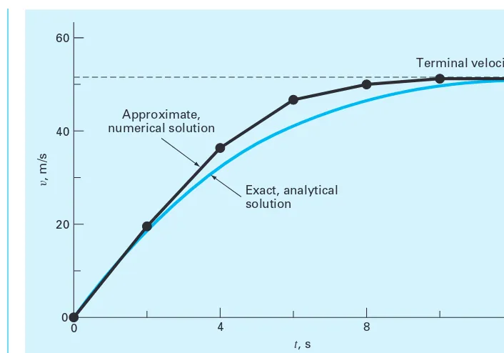
The results are plotted in Fig. 1.4 along with the exact solution. We can see that the nu-merical method captures the essential features of the exact solution. However, because we have employed straight-line segments to approximate a continuously curving function, there is some discrepancy between the two results. One way to minimize such discrepan-cies is to use a smaller step size. For example, applying Eq. (1.12) at 1-s intervals results in a smaller error, as the straight-line segments track closer to the true solution. Using hand calculations, the effort associated with using smaller and smaller step sizes would make such numerical solutions impractical. However, with the aid of the computer, large num-bers of calculations can be performed easily. Thus, you can accurately model the velocity of the jumper without having to solve the differential equation exactly.
1.1 A SIMPLE MATHEMATICAL MODEL 11
0 20 40 60
0 4 8 12
t, s
Terminal velocity
v
, m/s
Approximate, numerical solution
[image:31.615.110.463.66.313.2]Exact, analytical solution
FIGURE 1.4
As in Example 1.2, a computational price must be paid for a more accurate numerical result. Each halving of the step size to attain more accuracy leads to a doubling of the num-ber of computations. Thus, we see that there is a trade-off between accuracy and computa-tional effort. Such trade-offs figure prominently in numerical methods and constitute an important theme of this book.
1.2 CONSERVATION LAWS IN ENGINEERING AND SCIENCE
Aside from Newton’s second law, there are other major organizing principles in science and engineering. Among the most important of these are the conservation laws. Although they form the basis for a variety of complicated and powerful mathematical models, the great conservation laws of science and engineering are conceptually easy to understand. They all boil down to
Change=increases−decreases (1.14)
This is precisely the format that we employed when using Newton’s law to develop a force balance for the bungee jumper [Eq. (1.8)].
Although simple, Eq. (1.14) embodies one of the most fundamental ways in which conservation laws are used in engineering and science—that is, to predict changes with respect to time. We will give it a special name—the time-variable(or transient) computation.
Aside from predicting changes, another way in which conservation laws are applied is for cases where change is nonexistent. If change is zero, Eq. (1.14) becomes
Change=0=increases−decreases or
Increases=decreases (1.15)
Thus, if no change occurs, the increases and decreases must be in balance. This case, which is also given a special name—the steady-state calculation—has many applications in engi-neering and science. For example, for steady-state incompressible fluid flow in pipes, the flow into a junction must be balanced by flow going out, as in
Flow in= o w out
For the junction in Fig. 1.5, the balance can be used to compute that the flow out of the fourth pipe must be 60.
For the bungee jumper, the steady-state condition would correspond to the case where the net force was zero or [Eq. (1.8) with dv/dt=0]
mg=cdv2 (1.16)
Thus, at steady state, the downward and upward forces are in balance and Eq. (1.16) can be solved for the terminal velocity
v=
gm
cd
Table 1.1 summarizes some models and associated conservation laws that figure promi-nently in engineering. Many chemical engineering problems involve mass balances for reactors. The mass balance is derived from the conservation of mass. It specifies that the change of mass of a chemical in the reactor depends on the amount of mass flowing in minus the mass flowing out.
Civil and mechanical engineers often focus on models developed from the conserva-tion of momentum. For civil engineering, force balances are utilized to analyze structures such as the simple truss in Table 1.1. The same principles are employed for the mechanical engineering case studies to analyze the transient up-and-down motion or vibrations of an automobile.
Finally, electrical engineering studies employ both current and energy balances to model electric circuits. The current balance, which results from the conservation of charge, is simi-lar in spirit to the flow balance depicted in Fig. 1.5. Just as flow must balance at the junction of pipes, electric current must balance at the junction of electric wires. The energy balance specifies that the changes of voltage around any loop of the circuit must add up to zero.
It should be noted that there are many other branches of engineering beyond chemical, civil, electrical, and mechanical. Many of these are related to the Big Four. For example, chem-ical engineering skills are used extensively in areas such as environmental, petroleum, and bio-medical engineering. Similarly, aerospace engineering has much in common with mechanical engineering. I will endeavor to include examples from these areas in the coming pages.
1.3 NUMERICAL METHODS COVERED IN THIS BOOK
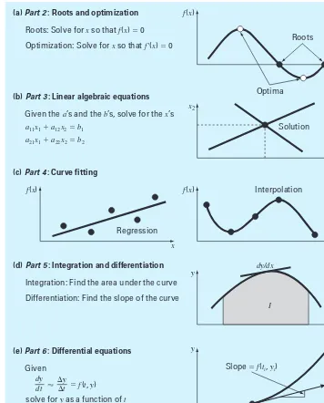
Euler’s method was chosen for this introductory chapter because it is typical of many other classes of numerical methods. In essence, most consist of recasting mathematical opera-tions into the simple kind of algebraic and logical operaopera-tions compatible with digital com-puters. Figure 1.6 summarizes the major areas covered in this text.
1.3 NUMERICAL METHODS COVERED IN THIS BOOK 13
Pipe 2
Flow in ⫽ 80
Pipe 3
Flow out ⫽ 120
Pipe 4
Flow out ⫽ ?
Pipe 1
Flow in ⫽ 100
FIGURE 1.5
TABLE 1.1 Devices and types of balances that are commonly used in the four major areas of engineering. For each case, the conservation law on which the balance is based is specified.
Field Device Organizing Principle Mathematical Expression
Force balance: Mechanical
engineering
Conservation of momentum
Upward force
Downward force
x⫽ 0
⫽ downward force ⫺ upward force
m d2x dt2
Machine
Current balance:
Voltage balance:
Around each loop
⌺ emf’s ⫺⌺ voltage drops for resistors
⫽ 0 ⌺ ⫺⌺ iR⫽ 0
For each node ⌺ current (i) ⫽ 0 Electrical
engineering
Conservation of energy Conservation of charge
⫹i2
⫺i3
⫹i1
i1R1
i3R3 i2R2
⫹ ⫺
Circuit Chemical
engineering
Conservation of mass
Over a unit of time period
⌬mass ⫽ inputs ⫺ outputs
Mass balance:
Reactors
Force balance:
At each node
⌺ horizontal forces (FH) ⫽ 0
⌺ vertical forces (FV) ⫽ 0
Civil engineering
Conservation of momentum
Structure
⫹FV
⫺FV
⫹FH
⫺FH
1.3 NUMERICAL METHODS COVERED IN THIS BOOK 15
⌬t
Slope ⫽ f(ti, yi)
y (e)Part 6: Differential equations
Given
solve for y as a function of t
dy dt
⌬y ⫽ ⌬t
⬇ f(t, y)
(c)Part 4: Curve fitting
(d)Part 5: Integration and differentiation
Integration: Find the area under the curve
Differentiation: Find the slope of the curve Regression
Interpolation
(a)Part 2:Roots and optimization
Roots: Solve for x so that f(x) ⫽ 0 Optimization: Solve for x so that f '(x) ⫽ 0
(b)Part 3: Linear algebraic equations
Given the a’s and the b’s, solve for the x’s
a11x1⫹ a12x2⫽b1 a21x1⫹ a22x2⫽b2
Solution Roots
Optima
x
x1
x x
x
t f(x)
x2
f(x)
f(x)
y
dy/dx
I
[image:35.615.122.478.71.513.2]yi⫹1⫽yi⫹f(ti, yi)⌬t
FIGURE 1.6
Part Twodeals with two related topics: root finding and optimization. As depicted in Fig. 1.6a, root locationinvolves searching for the zeros of a function. In contrast, optimiza-tioninvolves determining a value or values of an independent variable that correspond to a “best” or optimal value of a function. Thus, as in Fig. 1.6a, optimization involves identify-ing maxima and minima. Although somewhat different approaches are used, root location and optimization both typically arise in design contexts.
Part Threeis devoted to solving systems of simultaneous linear algebraic equations (Fig. 1.6b). Such systems are similar in spirit to roots of equations in the sense that they are concerned with values that satisfy equations. However, in contrast to satisfying a single equation, a set of values is sought that simultaneously satisfies a set of linear algebraic equations. Such equations arise in a variety of problem contexts and in all disciplines of en-gineering and science. In particular, they originate in the mathematical modeling of large systems of interconnected elements such as structures, electric circuits, and fluid networks. However, they are also encountered in other areas of numerical methods such as curve fit-ting and differential equations.
As an engineer or scientist, you will often have occasion to fit curves to data points. The techniques developed for this purpose can be divided into two general categories: regression and interpolation. As described in Part Four (Fig. 1.6c), regression is employed where there is a significant degree of error associated with the data. Experi-mental results are often of this kind. For these situations, the strategy is to derive a sin-gle curve that represents the general trend of the data without necessarily matching any individual points.
In contrast, interpolationis used where the objective is to determine intermediate val-ues between relatively error-free data points. Such is usually the case for tabulated infor-mation. The strategy in such cases is to fit a curve directly through the data points and use the curve to predict the intermediate values.
As depicted in Fig. 1.6d, Part Five is devoted to integration and differentiation. A physical interpretation of numerical integrationis the determination of the area under a curve. Integration has many applications in engineering and science, ranging from the determination of the centroids of oddly shaped objects to the calculation of total quan-tities based on sets of discrete measurements. In addition, numerical integration formu-las play an important role in the solution of differential equations. Part Five also covers methods for numerical differentiation. As you know from your study of calculus, this involves the determination of a function’s slope or its rate of change.
1.4 CASE STUDY IT’S A REAL DRAG
1.4 CASE STUDY 17
Background. In our model of the free-falling bungee jumper, we assumed that drag depends on the square of velocity (Eq. 1.7). A more detailed representation, which was originally formulated by Lord Rayleigh, can be written as
Fd = −1 2ρv
2ACdv (1.17)
where Fd⫽the drag force (N), ⫽fluid density (kg/m3), A⫽the frontal area of the object
on a plane perpendicular to the direction of motion (m2), C
d⫽a dimensionless drag
coef-ficient, and v⫽a unit vector indicating the direction of velocity.
This relationship, which assumes turbulent conditions (i.e., a high Reynolds number), allows us to express the lumped drag coefficient from Eq. (1.7) in more fundamental terms as
Cd = 1
2ρACd (1.18)
Thus, the lumped drag coefficient depends on the object’s area, the fluid’s density, and a dimensionless drag coefficient. The latter accounts for all the other factors that contribute to air resistance such as the object’s “roughness”. For example, a jumper wearing a baggy outfit will have a higher Cdthan one wearing a sleek jumpsuit.
Note that for cases where velocity is very low, the flow regime around the object will be laminar and the relationship between the drag force and velocity becomes linear. This is referred to as Stokes drag.
In developing our bungee jumper model, we assumed that the downward direction was positive. Thus, Eq. (1.7) is an accurate representation of Eq. (1.17), because v⫽ ⫹1 and the drag force is negative. Hence, drag reduces velocity.
But what happens if the jumper has an upward (i.e., negative) velocity? In this case,
v⫽–1 and Eq. (1.17) yields a positive drag force. Again, this is physically correct as the pos-itive drag force acts downward against the upward negative velocity.
Unfortunately, for this case, Eq. (1.7) yields a negative drag force because it does not include the unit directional vector. In other words, by squaring the velocity, its sign and hence its direction is lost. Consequently, the model yields the physically unrealistic result that air resistance acts to accelerate an upward velocity!
In this case study, we will modify our model so that it works properly for both downward and upward velocities. We will test the modified model for the same case as Example 1.2, but with an initial value of v(0) ⫽⫺40 m/s. In addition, we will also illustrate how we can extend the numerical analysis to determine the jumper’s position.
Solution. The following simple modification allows the sign to be incorporated into the drag force:
Fd = −
1
1.4 CASE STUDY continued
or in terms of the lumped drag:
Fd = −cdv|v| (1.20)
Thus, the differential equation to be solved is
dv
dt =g− cd
mv|v| (1.21)
In order to determine the jumper’s position, we recognize that distance travelled,
x(m), is related to velocity by
d x
dt = −v (1.22)
In contrast to velocity, this formulation assumes that upward distance is positive. In the same fashion as Eq. (1.12), this equation can be integrated numerically with Euler’s method:
xi+1=xi−v(ti)t (1.23)
Assuming that the jumper’s initial position is defined as x(0) ⫽0, and using the parame-ter values from Examples 1.1 and 1.2, the velocity and distance at t⫽2 s can be computed as
v(2)= −40+
9.81−0.25
68.1(−40)(40)
2= −8.6326 m/s
x(2)=0−(−40)2=80 m
Note that if we had used the incorrect drag formulation, the results would be ⫺32.1274 m/s and 80 m.
The computation can be repeated for the next interval (t⫽2 to 4 s):
v(4)= −8.6326+
9.81−0.25
68.1(−8.6326)(8.6326)
2=11.5346 m/s
x(4)=80−(−8.6326)2=97.2651 m
The incorrect drag formulation gives –20.0858 m/s and 144.2549 m.
The calculation is continued and the results shown in Fig. 1.7 along with those obtained with the incorrect drag model. Notice that the correct formulation decelerates more rapidly because drag always diminishes the velocity.
With time, both velocity solutions converge on the same terminal velocity because eventually both are directed downward in which case, Eq. (1.7) is correct. However, the impact on the height prediction is quite dramatic with the incorrect drag case resulting in a much higher trajectory.
1.4 CASE STUDY 19
1.4 CASE STUDY continued
FIGURE 1.7
Plots of (a) velocity and (b) height for the free-falling bungee jumper with an upward (negative) initial velocity generated with Euler’s method. Results for both the correct (Eq. 1 20) and incorrect (Eq. 1.7) drag formulations are displayed.
v
, m/s
0 20 40
–40 –20
60
4 8 12
t, s Correct drag
Incorrect drag
(a) Velocity, m/s
(b) Height, m
0 100 200
–200 –100
4 8 12
t, s
x
, m
Incorrect drag
PROBLEMS
1.1 Use calculus to verify that Eq. (1.9) is a solution of Eq. (1.8) for the initial condition v(0) ⫽0.
1.2 Use calculus to solve Eq. (1.21) for the case where the ini-tial velocity is (a)positive and (b)negative. (c)Based on your results for (a) and (b), perform the same computation as in Ex-ample 1.1 but with an initial velocity of ⫺40 m/s. Compute values of the velocity from t⫽0 to 12 s at intervals of 2 s. Note that for this case, the zero velocity occurs at t⫽3.470239 s. 1.3 The following information is available for a bank account:
Date Deposits Withdrawals Balance
5/1 1512.33 220.13 327.26 6/1 216.80 378.61 7/1 450.25 106.80 8/1 127.31 350.61 9/1
Note that the money earns interest which is computed as
Interest=i Bi
where i⫽the interest rate expressed as a fraction per month, and Bithe initial balance at the beginning of the month. (a) Use the conservation of cash to compute the balance on
6/1, 7/1, 8/1, and 9/1 if the interest rate is 1% per month (i⫽0.01/month). Show each step in the computation. (b) Write a differential equation for the cash balance in the
form
d B
dt = f[D(t),W(t),i]
where t⫽time (months), D(t) ⫽deposits as a function of time ($/month), W(t) ⫽withdrawals as a function of time ($/month). For this case, assume that interest is compounded continuously; that is, interest ⫽iB.
(c) Use Euler’s method with a time step of 0.5 month to simulate the balance. Assume that the deposits and with-drawals are applied uniformly over the month.
(d) Develop a plot of balance versus time for (a)and (c). 1.4 Repeat Example 1.2. Compute the velocity to t=12 s, with a step size of (a)1 and (b)0.5 s. Can you make any statement regarding the errors of the calculation based on the results?
1.5 Rather than the nonlinear relationship of Eq. (1.7), you might choose to model the upward force on the bungee jumper as a linear relationship:
FU = −c′v
where c′=a first-order drag coefficient (kg/s).
(a) Using calculus, obtain the closed-form solution for the case where the jumper is initially at rest (v=0 at t=0). (b) Repeat the numerical calculation in Example 1.2 with
the same initial condition and parameter values. Use a value of 11.5 kg/s for c′.
1.6 For the free-falling bungee jumper with linear drag (Prob. 1.5), assume a first jumper is 70 kg and has a drag co-efficient of 12 kg/s. If a second jumper has a drag coco-efficient of 15 kg/s and a mass of 80 kg, how long will it take her to reach the same velocity jumper 1 reached in 9 s?
1.7 For the second-order drag model (Eq. 1.8), compute the velocity of a free-falling parachutist using Euler’s method for the case where m=80 kg and cd=0.25 kg/m. Perform
the calculation from t=0 to 20 s with a step size of 1 s. Use an initial condition that the parachutist has an upward veloc-ity of 20 m/s at t=0. At t=10 s, assume that the chute is instantaneously deployed so that the drag coefficient jumps to 1.5 kg/m.
1.8 The amount of a uniformly distributed radioactive con-taminant contained in a closed reactor is measured by its concentrationc(becquerel/liter or Bq/L). The contaminant decreases at a decay rate proportional to its concentration; that is
Decay rate= −kc
where kis a constant with units of day−1. Therefore, accord-ing to Eq. (1.14), a mass balance for the reactor can be written as
dc
dt = −kc
change in mass = decrease by decay
(a) Use Euler’s method to solve this equation from t=0 to 1 d with k=0.175 d–1. Employ a step size of
t=0.1 d. The concentration at t=0 is 100 Bq/L.
(b) Plot the solution on a semilog graph (i.e., ln cversus t) and determine the slope. Interpret your results. 1.9 A storage tank (Fig. P1.9) contains a liquid at depth y
PROBLEMS 21 0 y FIGURE P1.9 0 y ytop yout rtop Qin s 1 Qout FIGURE P1.11
resupplied at a sinusoidal rate 3Qsin2(
t). Equation (1.14) can be written for this system as
d(Ay)
dt =3Qsin
2
(t)− Q
change in
volume
= (in o w) −(out o w)
or, since the surface area Ais constant
d y dt =3
Q Asin
2(t)− Q
A
Use Euler’s method to solve for the depth yfrom t=0 to 10 d with a step size of 0.5 d. The parameter values are A=
1250 m2and Q=450 m3/d. Assume that the initial condition is y=0.
1.10 For the same storage tank described in Prob. 1.9, sup-pose that the outflow is not constant but rather depends on the depth. For this case, the differential equation for depth can be written as
d y dt =3
Q Asin
2(t)−α(1+y)1.5
A
Use Euler’s method to solve for the depth yfrom t=0 to 10 d with a step size of 0.5 d. The parameter values are A=
1250 m2,
Q=450 m3/d, and
α=150. Assume that the ini-tial condition is y=0.
1.11 Apply the conservation of volume (see Prob. 1.9) to sim-ulate the level of liquid in a conical storage tank (Fig. P1.11).
The liquid flows in at a sinusoidal rate of Qin=3 sin 2(
t) and flows out according to
Qout=3(y−yout)1.5 y>yout
Qout=0 y≤yout where flow has units of m3/d and
y=the elevation of the water surface above the bottom of the tank (m). Use Euler’s method to solve for the depth yfrom t=0 to 10 d with a step size of 0.5 d. The parameter values are rtop⫽2.5 m, ytop⫽4 m, and yout⫽1 m. Assume that the level is initially below the outlet pipe with y(0) ⫽0.8 m.
1.12 A group of 35 students attend a class in an insulated room which measures 11 m by 8 m by 3 m. Each student takes up about 0.075 m3and gives out about 80 W of heat (1 W=1 J/s). Calculate the air temperature rise during the first 20 minutes of the class if the room is completely sealed and in-sulated. Assume the heat capacityCvfor air is 0.718 kJ/(kg K).
Assume air is an ideal gas at 20°C and 101.325 kPa. Note that the heat absorbed by the air Qis related to the mass of the air mthe heat capacity, and the change in temperature by the following relationship:
Q=m
T2
T1
Cvd T=mCv(T2−T1)
The mass of air can be obtained from the ideal gas law:
P V = m
MwtRT
FIGURE P1.16 Q1 Q10 Q2 Q3 Q9 Q4 Q5 Q8
Q6 Q7
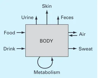
1.13 Figure P1.13 depicts the various ways in which an aver-age man gains and loses water in one day. One liter is ingested as food, and the body metabolically produces 0.3 liters. In breathing air, the exchange is 0.05 liters while inhaling, and 0.4 liters while exhaling over a one-day period. The body will also lose 0.3, 1.4, 0.2, and 0.35 liters through sweat, urine, feces, and through the skin, respectively. To maintain steady state, how much water must be drunk per day?
1.14 In our example of the free-falling bungee jumper, we assumed that the acceleration due to gravity was a constant value of 9.81 m/s2. Although this is a decent approximation when we are examining falling objects near the surface of the earth, the gravitational force decreases as we move above sea level. A more general representation based on Newton’s inverse square law of gravitational attraction can be written as
g(x)=g(0) R
2
(R+x)2
where g(x) =gravitational acceleration at altitude x(in m) measured upward from the earth’s surface (m/s2),
g(0) =
gravitational acceleration at the earth’s surface (∼=9.81 m/s2), and R=the earth’s radius (∼=6.37 ×10⁶m).
(a) In a fashion similar to the derivation of Eq. (1.8), use a force balance to derive a differential equation for veloc-ity as a function of time that utilizes this more complete representation of gravitation. However, for this deriva-tion, assume that upward velocity is positive.
(b) For the case where drag is negligible, use the chain rule to express the differential equation as a function of alti-tude rather than time. Recall that the chain rule is
dv dt = dv