VORONOI DIAGRAMS WITHOUT BOUNDING BOXES
Erik Tjong Kim Sang
Meertens Institute, The Netherlands, [email protected]
KEY WORDS: Voronoi Diagrams, Maps, Languages, Dialects
ABSTRACT:
We present a technique for presenting geographic data in Voronoi diagrams without having to specify a bounding box. The method restricts Voronoi cells to points within a user-defined distance of the data points. The mathematical foundation of the approach is presented as well. The cell clipping method is particularly useful for presenting geographic data that is spread in an irregular way over a map, as for example the Dutch dialect data displayed in Figure 2. The automatic generation of reasonable cell boundaries also makes redundant a frequently used solution to this problem that requires data owners to specify region boundaries, as in Goebl (2010) and Nerbonne et al (2011).
1. INTRODUCTION
We have a developed a free online tool for quickly displaying geographic data on a map1. The tool uses standards such as OpenLayers and OpenStreepMap for background maps and navigation, and csv and kml for data files. It is programmed in Javascript, a standard language for web applications. Users can upload geographic data consisting of coordinates linked to numbers or strings and these will be displayed as categories with colours. The tool is currently primarily used for creating maps of the geographic spread of dialect variants of various human languages.
The tool displays geographic data using Voronoi diagrams, divisions of maps in cells such that each point in the map is part of a cell with points, that are closer to a particular data point than to any other data point. An example of such a diagram can be found in Figure 1. The four points in the graph are the four data points. The other points in the area have been divided over four cells such that each point lies in the same cell as the closest data point. A predefined rectangular area drawn around the data points, the bounding box, restricts the size of the four cells.
Figure 1. Basic Voronoi diagram with four data points. The area is divided in four cells of points, that are closest to each data point. The size of the cells is limited by a predefined rectangular area, the bounding box. We would like the cells to be restricted by a maximum size rather than a predefined rectangle.
1 http://ifarm.nl/maps/arvid
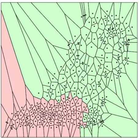
We use Voronoi diagrams for visualizing geographic data. Such data points are often spread over a map in an irregular way. For this type of data a rectangular bounding box is not appropriate. Figure 2 gives an example of a geographic data set2 in a Voronoi diagram with a rectangular shaped bounding box. The color of a Voronoi cell indicates what type of dialect is spoken in the area covered by the cell. However, because of the shape of the bounding box, the left-most and right-most cells are much larger than the other cells. This is undesirable because the big cells cover areas that are much larger than can be implied from the data. For example, this data set covers areas in The Netherlands and Belgium where the language Dutch is spoken. Because of the shape of the bounding box, the right-most areas extend far into Germany, where no Dutch is spoken.
Figure 2. Voronoi diagram for geographic data. The bounding box is not appropriate for this irregularly spread data. It makes
2 The Dutch dialect data in Figures 2, 3 and 6 are an aggregated
version of the data in the SAND database (Barbiers et al, 2006).
the left-most and right-most cells very large, leading to incorrect conclusions about the areas covered by the data points.
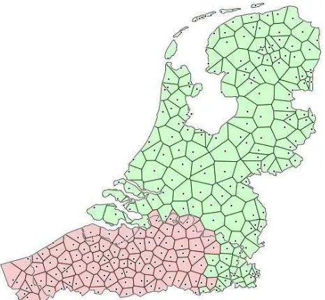
A common approach for obtaining nice Voronoi maps with geographic data is to use region boundaries from an external map as bounding box (Figure 3). However, relevant boundaries might not always be available. This is certainly true for our tool, where users can supply any data set. We do not want to require them to define region boundaries for their data. Therefore we are looking for an automatic method for restricting the cells of a Voronoi diagram. In this paper describe such a method.
The contribution of this paper is an algorithm for automatically determining reasonable outer boundaries of a Voronoi diagram, without the need of an artificial bounding box or predefined region outlines, and without the restriction of the data points to fit in a convex shape. Javascript code implementing this algorithm can be found at our visualization tool page1.
After this introduction, we will describe related work. In section 3, we introduce the problem and present the general steps that can be taken for solving it. Some of the solution steps require mathematical computations and the relevant formulas are presented in section 4. In the final section, we give some reasonable sizes. However, not every data set corresponds with
3 The Voronoi diagram with region boundaries was created with
the package RuG-L04, written by Peter Kleiweg.
existing geographical regions. Visualizing data in this way may require the data provider to supply relevant region boundaries as well.
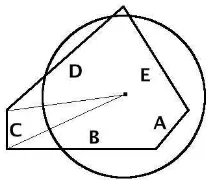
Figure 4. Voronoi cell with five sides (ABCDE) with the data point and a bounding circle. Our goal is to restrict the size of the polygon to the points lying inside the circle. Edge A will be kept, edge C will be discarded and usage of edges B, D and E will be restricted to the parts of them that lie inside the circle.
diagrams and similar data models include among others material physics (Sze and Ng, 2006), robot navigation (Thrun, 1998) and epidemiology (Snow, 1855). In our field, studying the geographic spread of the dialect variants of human languages, Voronoi diagrams are most famously used in the work of Hans Goebl and colleagues in Salzburg, who apply them for creating several dialect maps of European regions (Goebl, 2010). For dialect maps, rectangular bounding boxes produce unsatisfactory maps and therefore such maps usually use region outlines as bounding boxes (Goebl, 2010) (Nerbonne et al, 2011). However, this puts an extra burden on the map users, who either need to restrict their work to predefined regions or define their own region outlines. The program Mathematica for scientific computations includes a package mPower (formerly Qhull) for generating bounded Voronoi cells for maps, that do not require a predefined bounding box (Barber et al, 1996). The package restricts the size of the generated cells by adding artificial data points around the original ones before computing the cells and removing them again after the computation. However, the approach creates convex spaces which may not always be appropriate for the data sets that we are working with. Gabmap (Nerbonne et al, 2011) has experimented with circular boundaries for border cells but these are not available in their demo anymore. The examples page on the website for Javascript library D3 links an example that uses the SVG function clipPath, that can be used for creating similar figures as the method described in this paper (Vack, 2011).
3. PROBLEM DESCRIPTION AND SOLUTION
We want to map geographic data using Voronoi diagrams. Rectangular bounding boxes are unsatisfactory for this purpose since the data are usually spread in an irregular way over the map. Region boundaries work well as boundaries for geographic data (Goebl, 2010). However, we will use the Voronoi diagrams for mapping arbitrary data of arbitrary users. Relevant region outlines might not be available and we do not want to put the burden on the data providers to supply such region boundaries. Barber et al (1996) outlined a method for automatically restricting the size of cells in a Voronoi diagram without the need for a bounding box. However, this method fits the data points in a convex shape. In our own data sets we have examples of concave sets of data points and even split sets. Therefore we cannot use the solution of Barber et al (1996). As ISPRS Annals of the Photogrammetry, Remote Sensing and Spatial Information Sciences, Volume II-2/W2, 2015
an alternative, we will use a post-processing method for clipping long polygon edges after building the Voronoi cells.
Figure 5. Mapping an edge (C) to the bounding circle: We draw straight lines from the vertices of the edge to the center of the circle and use the intersection points of these lines and the circle as the two end points of the new line.
Figure 4 gives an example of a Voronoi cell (the pentagon) of which we want to restrict the distance between its vertices (corner points) and the data point. The circle shows the target maximum size of the cell. In our visualisation tool the diameter of this circle is a value which is determined by the user. The five cell edges are examples of the possible edge variants with respect to the circle limit:
an edge may lay completely inside the bounding circle, as for example edge A
an edge may lay completely outside the bounding circle, as for example edge C
an edge may have one intersection with the bounding circle, as for example edges B and E
an edge may have two intersections with the bounding circle, as for example edge D
Our goal is to transform the polygon to one that completely lies inside the circle. We will use all polygon edge parts that lie inside the circle. We will replace the polygon edge parts that lie outside the circle with an approximation of the corresponding circle boundary. This means that we will perform the following actions for the edge variants:
edges completely inside the bounding circle (edge A): use them
edges completely outside the bounding circle (C): replace the complete edge by its corresponding circle part
edges with one intersection with the bounding circle (B and E): use the part inside the circle, replace the rest with the corresponding circle part
edges with two intersections with the bounding circle (D): use the part inside the circle, replace the other two parts by their corresponding circle part
Figure 5 shows what we mean with the corresponding circle part: we draw straight lines from the two vertices of an edge to the data point. The intersections of these lines and the circle mark the start and end point of the circle part that corresponds with the original line. As far as we know, our software cannot draw polygons with circle parts. Therefore, we map many points of each edge to the circle. When the corresponding intersecting points are connected they form an approximation of the corresponding part of the circle.
4. COMPUTING NEW CELL VERTICES
Restricting the size of polygons requires some computations. First, we need to test if a vertex of a cell lies inside the bounding circle. We do this by computing the distance of the vertex to the circle center and comparing it with the circle radius:
distance(P,Center)= (Px- Centerx) 2+ the circle, as shown in Figure 5 for the vertices of edge C. We do this by changing the x coordinate and the y coordinate in compute the distance of the new point NewP to the circle center with Equation (1) by replacing the coordinates Px and Py with the right hand sides of Equations (2) and (3), we obtain: distance(NewP,Center) = Radius.
Finally, we need to determine the intersection points of polygon edges and the bounding circle. Examples of these points are the intersections of lines B, D and E with the circle in Figure 5. Of each edge we know only the two vertices as a result of the Voronoi algorithm. We start with creating a definition of the points on the straight line corresponding to an edge:
y = a*x + b with a = (y2-y1) / (x2-x1) and b = (y1*x2-y2*x1)/(x2-x1) (4)
Here (x1,y1) and (x2,y2) are the coordinates of the two vertices. The equation y = a*x + b describes the unique straight line through these two points. This equation cannot describe vertical lines (x2 = x1). For those we need an alternative but similar equation x = a*y + b where a = 0 and b = x1.
Next, we create a definition of the bounding circle:
y=Centery± Radius
Next we combine the circle equation (5) with the line equation (4) to find the intersection points of a line and a circle. Both equations have a right hand side equal to y so the two right hand sides are equal to each other:
Centery± Radius
2- (x- Center x)
2=a*x+b
(6)
We subtract Centery from the left and right side and square both results:
Next we expand all squares. Our target is a quadratic equation of the form A*x2+ B*x+ C= 0: corresponding values of x with the standard formula for solving
quadratic equations: x= - B± B
2- 4 *A*C
2 *A . Next we can
compute the associated values of y with the line equation (4), which gives us the coordinates of the intersecting points of the circle and the line, if there are any. The quadratic equation has two solutions (two intersecting points) if B2> 4*A*C, one solution if B2= 4*A*C and no solutions if B2< 4*A*C. From the intersection points, we can determine the new boundaries of the cells.
All computations for a vertex of a cell are independent from the computations for the other vertices so we estimate the complexity of the computations as O(n), where n is the number of edges in the Voronoi diagram.
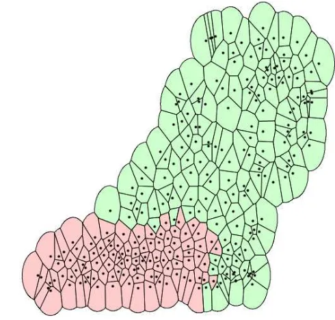
Figure 6. A Voronoi map of the Dutch language area after being processed with the cell edge clipping method described in this paper. The smaller cells after edge clipping are a better approximation of the dialect areas than the cells associated with the rectangular bounding box displayed in Figure 2.
5. CONCLUDING REMARKS
We have presented a method for restricting the sizes of the cells of a Voronoi diagram without having to rely on an overall bounding box. The method restricts all the cell edges to points that are not further away from the corresponding data point than a user-defined distance D. The cut edges are then connected by a set of line segments that approximate the bounding circle with radius D around the data point. We have presented a general description of the method (Section 3), a technical outline of how to compute the relevant points (Section 4). The method works well, as can be seen in Figure 6. It is currently being used for analysing irregularly shaped disjoint dialect regions. We hope that approach will be useful for other researchers that use Voronoi maps for visualizing geographic data.
REFERENCES
Aurenhammer, F., Klein, R. and Lee, D.T., 2013. Voronoi Diagrams and Delaunay Triangulations. World Scientific Publishing. ISBN 978-9814447638.
Barber, C.B., Dobkin D.P., and Huhdanpaa, H.T., 1996. The quickhull algorithm for convex hulls. ACM Transactions on Mathematical Software, 22(4):469–483.
Barbiers, S., 2006. Dynamic Syntactic Atlas of the Dutch Dialects (DynaSand). Amsterdam, Meertens Institute.
http://www.meertens.knaw.nl/sand/ . Retrieved 19 August 2015.
Goebl, H., 2010. Dialectometry: Theoretical prerequisites, practical problems and concrete applications. Dialectologia, Special Issue(I):63–77.
Hill, R., 2010. Javascript-voronoi. Javascript module available
at http://github.com/gorhill/Javascript-Voronoi . Retrieved 6
May 2015.
Nerbonne, J., Colen, R., Gooskens, C., Kleiweg, P. and Leinonen, T., 2011. Gabmap – a web application for dialectology. Dialectologia, Special Issue(II):65–89.
Snow, J., 1855, On the mode of communication of cholera. John Churchill.
Sze, S.M. and Ng, K.K., 2006. Physics of Semiconductor Devices. John Wiley & Sons.
Thrun, S., 1998. Learning metric-topological maps for indoor mobile robot navigation. Artificial Intelligence, 99(1), 21-71.
Vack, N., 2011. Voronoi-based point picker. Javascript example of round points restricted by Voronoi cells at
http://bl.ocks.org/njvack/1405439 . Retrieved 18 August 2015.
Voronoï, G., 1908. Nouvelles applications des paramètres continus à la théorie des formes quadratiques. Journal für die reine angewandte Mathematik, 1908(134):198–287.