Programming Embedded Systems in C and C++
Michael Barr
Publisher: O'Reilly
First Edition January 1999 ISBN: 1-56592-354-5, 191 pages
Why I Wrote This Book
I once heard an estimate that in the United States there are eight microprocessor-based devices for every person. At the time, I wondered how this could be. Are there really that many computers surrounding us? Later, when I had more time to think about it, I started to make a list of the things I used that probably contained a microprocessor. Within five minutes, my list contained ten items: television, stereo, coffee maker, alarm clock, VCR, microwave, dishwasher, remote control, bread machine, and digital watch. And those were just my personal possessions-I quickly came up with ten more devices I used at work.
The revelation that every one of those products contains not only a processor, but also software, was not far behind. At last, I knew what I wanted to do with my life. I wanted to put my programming skills to work developing
embedded computer systems. But how would I acquire the necessary knowledge? At this point, I was in my last year of college. There hadn't been any classes on embedded systems programming so far, and I wasn't able to find any listed in the course catalog.
Fortunately, when I graduated I found a company that let me write embedded software while I was still learning. But I was pretty much on my own. The few people who knew about embedded software were usually too busy to explain things to me, so I searched high and low for a book that would teach me. In the end, I found I had to learn
everything myself. I never found that book, and I always wondered why no one had written it.
Intended Audience
This is a book about programming embedded systems in C and C++. As such, it assumes that the reader already has some programming experience and is at least familiar with the syntax of these two languages. It also helps if you have some familiarity with basic data structures, such as linked lists. The book does not assume that you have a great deal of knowledge about computer hardware, but it does expect that you are willing to learn a little bit about hardware along the way. This is, after all, a part of the job of an embedded programmer.
While writing this book, I had two types of readers in mind. The first reader is a beginner-much as I was when I graduated from college. She has a background in computer science or engineering and a few years of programming experience. The beginner is interested in writing embedded software for a living but is not sure just how to get started. After reading the first five chapters, she will be able to put her programming skills to work developing simple embedded programs. The rest of the book will act as her reference for the more advanced topics encountered in the coming months and years of her career.
The second reader is already an embedded systems programmer. She is familiar with embedded hardware and knows how to write software for it but is looking for a reference book that explains key topics. Perhaps the embedded systems programmer has experience only with assembly language programming and is relatively new to C and C++. In that case, the book will teach her how to use those languages in an embedded system, and the later chapters will provide the advanced material she requires.
Organization
The book contains ten chapters, one appendix, a glossary, and an annotated bibliography. The ten chapters can be divided quite nicely into two parts. The first part consists of Chapter 1 through Chapter 5 and is intended mainly for newcomers to embedded systems. These chapters should be read in their entirety and in the order that they appear. This will bring you up to speed quickly and introduce you to the basics of embedded software development. After completingChapter 5, you will be ready to develop small pieces of embedded software on your own.
The second part of the book consists of Chapter 6 through Chapter 10 and discusses advanced topics that are of interest to inexperienced and experienced embedded programmers alike. These chapters are mostly self-contained and can be read in any order. In addition, Chapter 6 through Chapter 9 contain example programs that might be useful to you on a future embedded software project.
• Chapter 1 introduces you to embedded systems. It defines the term, gives examples, and explains why C
and C++ were selected as the languages of the book.
• Chapter 2 walks you through the process of writing a simple embedded program in C. This is roughly the
equivalent of the "Hello, World" example presented in most other programming books.
• Chapter 3 introduces the software development tools you will be using to prepare your programs for
execution by an embedded processor.
• Chapter 4 presents various techniques for loading your executable programs into an embedded system. It
also describes the debugging tools and techniques that are available to you.
• Chapter 5 outlines a simple procedure for learning about unfamiliar hardware platforms. After completing
this chapter, you will be ready to write and debug simple embedded programs.
• Chapter 6 tells you everything you need to know about memory in embedded systems. The chapter includes
source code implementations of memory tests and Flash memory drivers.
• Chapter 7 explains device driver design and implementation techniques and includes an example driver for
a common peripheral called a timer.
• Chapter 8 includes a very basic operating system that can be used in any embedded system. It also helps
you decide if you'll need an operating system at all and, if so, whether to buy one or write your own.
• Chapter 9 expands on the device driver and operating system concepts presented in the previous chapters. It
explains how to control more complicated peripherals and includes a complete example application that pulls together everything you've learned so far.
• Chapter 10 explains how to simultaneously increase the speed and decrease the memory requirements of
your embedded software. This includes tips for taking advantage of the most beneficial C++ features without paying a significant performance penalty.
Conventions, Typographical and Otherwise
The following typographical conventions are used throughout the book:
Italic
is used for the names of files, functions, programs, methods, routines, and options when they
appear in the body of a paragraph. Italic is also used for emphasis and to introduce new
terms.
Constant Width
is used in the examples to show the contents of files and the output of commands. In the body
of a paragraph, this style is used for keywords, variable names, classes, objects, parameters,
and other code snippets.
Constant Width Bold
is used in the examples to show commands and options that you type literally.
is used in the examples to show commands and options that you type literally.
This symbol is used to indicate a tip, suggestion, or general note.
This symbol is used to indicate a warning.
Other conventions relate to gender and roles. With respect to gender, I have purposefully
alternated my use of the terms "he" and "she" throughout the book. "He" is used in the
odd-numbered chapters and "she" in all of the even-odd-numbered ones.
With respect to roles, I have occasionally distinguished between the tasks of hardware engineers,
embedded software engineers, and application programmers in my discussion. But these titles
refer only to roles played by individual engineers, and it should be noted that it can and often
does happen that one individual fills more than one of these roles.
Obtaining the Examples Online
This book includes many source code listing, and all but the most trivial one-liners are available online. These examples are organized by chapter number and include build instructions (makefiles) to help you recreate each of the executables. The complete archive is available via FTP, at
How to Contact Us
We have tested and verified all the information in this book to the best of our ability, but you may find that features have changed (or even that we have made mistakes!). Please let us know about any errors you find, as well as your suggestions for future editions, by writing to:
O'Reilly & Associates
1005 Gravenstein Highway North
Sebastopol, CA 95472
800-998-9938 (in the U.S. or Canada)
707-829-0515 (international/local)
707-829-0104 (FAX)
You can also send us messages electronically. To be put on the mailing list or request a catalog, send email to:
To ask technical questions or comment on the book, send email to:
We have a web site for the book, where we'll list examples, errata, and any plans for future editions. You can access this page at:
http://www.oreilly.com/catalog/embsys/
For more information about this book and others, see the O'Reilly web site:
Personal Comments and Acknowledgments
As long as I can remember I have been interested in writing a book or two. But now that I have done so, I must confess that I was naive when I started. I had no idea how much work it would take, nor how many other people would have to get involved. Another thing that surprised me was how easy it was to find a willing publisher. I had expected that to be the hard part.
From proposal to publication, this project has taken almost two years to complete. But, then, that's mostly because I worked a full-time job throughout and tried to maintain as much of my social life as possible. Had I known when I started that I'd still be agonizing over final drafts at this late date, I would have probably quit working and finished the book more quickly. But continuing to work has been good for the book (as well as my bank account!). It has allowed me the luxury of discussing my ideas regularly with a complete cast of embedded hardware and software professionals. Many of these same folks have also contributed to the book more directly by reviewing drafts of some or all of the chapters.
I am indebted to all of the following people for sharing their ideas and reviewing my work: Toby Bennett, Paul Cabler (and the other great folks at Arcom), Mike Corish, Kevin D'Souza, Don Davis, Steve Edwards, Mike Ficco, Barbara Flanagan, Jack Ganssle, Stephen Harpster (who christened me "King of the Sentence Fragment" after reading an early draft), Jonathan Harris, Jim Jensen, Mark Kohler, Andy Kollegger, Jeff Mallory, Ian Miller, Henry Neugauss, Chris Schanck, Brian Silverman, John Snyder, Jason Steinhorn (whose constant stream of grammatical and technical critiques have made this book worth reading), Ian Taylor, Lindsey Vereen, Jeff Whipple, and Greg Young.
I would also like to thank my editor, Andy Oram. Without his enthusiasm for my initial proposal, overabundant patience, and constant encouragement, this book would never have been completed.
Chapter 1.
Introduction
I think there is a world market for maybe five computers.
-Thomas Watson, Chairman of IBM, 1943
There is no reason anyone would want a computer in their home.
-Ken Olson, President of Digital Equipment Corporation, 1977
One of the more surprising developments of the last few decades has been the ascendance of computers to a position of prevalence in human affairs. Today there are more computers in our homes and offices than there are people who live and work in them. Yet many of these computers are not recognized as such by their users. In this chapter, I'll explain what embedded systems are and where they are found. I will also introduce the subject of embedded programming, explain why I have selected C and C++ as the languages for this book, and describe the hardware used in the examples.
1.1 What Is an Embedded System?
Anembedded system is a combination of computer hardware and software, and perhaps additional mechanical or other parts, designed to perform a specific function. A good example is the microwave oven. Almost every
household has one, and tens of millions of them are used every day, but very few people realize that a processor and software are involved in the preparation of their lunch or dinner.
This is in direct contrast to the personal computer in the family room. It too is comprised of computer hardware and software and mechanical components (disk drives, for example). However, a personal computer is not designed to perform a specific function. Rather, it is able to do many different things. Many people use the term general-purpose computer to make this distinction clear. As shipped, a general-purpose computer is a blank slate; the manufacturer does not know what the customer will do with it. One customer may use it for a network file server, another may use it exclusively for playing games, and a third may use it to write the next great American novel.
Frequently, an embedded system is a component within some larger system. For example, modern cars and trucks contain many embedded systems. One embedded system controls the anti-lock brakes, another monitors and controls the vehicle's emissions, and a third displays information on the dashboard. In some cases, these embedded systems are connected by some sort of a communications network, but that is certainly not a requirement.
At the possible risk of confusing you, it is important to point out that a general-purpose computer is itself made up of numerous embedded systems. For example, my computer consists of a keyboard, mouse, video card, modem, hard drive, floppy drive, and sound card-each of which is an embedded system. Each of these devices contains a processor and software and is designed to perform a specific function. For example, the modem is designed to send and receive digital data over an analog telephone line. That's it. And all of the other devices can be summarized in a single sentence as well.
If an embedded system is designed well, the existence of the processor and software could be completely unnoticed by a user of the device. Such is the case for a microwave oven, VCR, or alarm clock. In some cases, it would even be possible to build an equivalent device that does not contain the processor and software. This could be done by replacing the combination with a custom integrated circuit that performs the same functions in hardware. However, a lot of flexibility is lost when a design is hard-coded in this way. It is much easier, and cheaper, to change a few lines of software than to redesign a piece of custom hardware.
1.1.1 History and Future
Given the definition of embedded systems earlier in this chapter, the first such systems could not possibly have appeared before 1971. That was the year Intel introduced the world's first microprocessor. This chip, the 4004, was designed for use in a line of business calculators produced by the Japanese company Busicom. In 1969, Busicom asked Intel to design a set of custom integrated circuits-one for each of their new calculator models. The 4004 was Intel's response. Rather than design custom hardware for each calculator, Intel proposed a general-purpose circuit that could be used throughout the entire line of calculators. This general-purpose processor was designed to read and execute a set of instructions-software-stored in an external memory chip. Intel's idea was that the software would give each calculator its unique set of features.
processors, and microwave ovens), living rooms (televisions, stereos, and remote controls), and workplaces (fax machines, pagers, laser printers, cash registers, and credit card readers) are embedded systems.
It seems inevitable that the number of embedded systems will continue to increase rapidly. Already there are promising new embedded devices that have enormous market potential: light switches and thermostats that can be controlled by a central computer, intelligent air-bag systems that don't inflate when children or small adults are present, palm-sized electronic organizers and personal digital assistants (PDAs), digital cameras, and dashboard navigation systems. Clearly, individuals who possess the skills and desire to design the next generation of embedded systems will be in demand for quite some time.
1.1.2 Real-Time Systems
One subclass of embedded systems is worthy of an introduction at this point. As commonly defined, areal-time system is a computer system that has timing constraints. In other words, a real-time system is partly specified in terms of its ability to make certain calculations or decisions in a timely manner. These important calculations are said to have deadlines for completion. And, for all practical purposes, a missed deadline is just as bad as a wrong answer.
The issue of what happens if a deadline is missed is a crucial one. For example, if the real-time system is part of an airplane's flight control system, it is possible for the lives of the passengers and crew to be endangered by a single missed deadline. However, if instead the system is involved in satellite communication, the damage could be limited to a single corrupt data packet. The more severe the consequences, the more likely it will be said that the deadline is "hard" and, thus, the system a hard real-time system. Real-time systems at the other end of this continuum are said to have "soft" deadlines.
All of the topics and examples presented in this book are applicable to the designers of real-time systems. However, the designer of a real-time system must be more diligent in his work. He must guarantee reliable operation of the software and hardware under all possible conditions. And, to the degree that human lives depend upon the system's proper execution, this guarantee must be backed by engineering calculations and descriptive paperwork.
1.2 Variations on the Theme
Unlike software designed for general-purpose computers, embedded software cannot usually be run on other embedded systems without significant modification. This is mainly because of the incredible variety in the underlying hardware. The hardware in each embedded system is tailored specifically to the application, in order to keep system costs low. As a result, unnecessary circuitry is eliminated and hardware resources are shared wherever possible. In this section you will learn what hardware features are common across all embedded systems and why there is so much variation with respect to just about everything else.
By definition all embedded systems contain a processor and software, but what other features do they have in common? Certainly, in order to have software, there must be a place to store the executable code and temporary storage for runtime data manipulation. These take the form of ROM and RAM, respectively; any embedded system will have some of each. If only a small amount of memory is required, it might be contained within the same chip as the processor. Otherwise, one or both types of memory will reside in external memory chips.
All embedded systems also contain some type of inputs and outputs. For example, in a microwave oven the inputs are the buttons on the front panel and a temperature probe, and the outputs are the human-readable display and the microwave radiation. It is almost always the case that the outputs of the embedded system are a function of its inputs and several other factors (elapsed time, current temperature, etc.). The inputs to the system usually take the form of sensors and probes, communication signals, or control knobs and buttons. The outputs are typically displays, communication signals, or changes to the physical world. See Figure 1-1 for a general example of an embedded system.
With the exception of these few common features, the rest of the embedded hardware is usually unique. This variation is the result of many competing design criteria. Each system must meet a completely different set of requirements, any or all of which can affect the compromises and tradeoffs made during the development of the product. For example, if the system must have a production cost of less than $10, then other things-like processing power and system reliability-might need to be sacrificed in order to meet that goal.
Of course, production cost is only one of the possible constraints under which embedded hardware designers work. Other common design requirements include the following:
Processing power
The amount of processing power necessary to get the job done. A common way to compare
processing power is the MIPS (millions of instructions per second) rating. If two processors
have ratings of 25 MIPS and 40 MIPS, the latter is said to be the more powerful of the two.
However, other important features of the processor need to be considered. One of these is the
register width, which typically ranges from 8 to 64 bits. Today's general-purpose computers
use 32- and 64-bit processors exclusively, but embedded systems are still commonly built
with older and less costly 8- and 16-bit processors.
Memory
The amount of memory (ROM and RAM) required to hold the executable software and the
data it manipulates. Here the hardware designer must usually make his best estimate up front
and be prepared to increase or decrease the actual amount as the software is being developed.
The amount of memory required can also affect the processor selection. In general, the
register width of a processor establishes the upper limit of the amount of memory it can
access (e.g., an 8-bit address register can select one of only 256 unique memory locations).
[1][1] Of course, the smaller the register width, the more likely it is that the processor employs tricks like
multiple address spaces to support more memory. A few hundred bytes just isn't enough to do much of anything. Several thousand bytes is a more likely minimum, even for an 8-bit processor.
Development cost
The cost of the hardware and software design processes. This is a fixed, one-time cost, so it
might be that money is no object (usually for high-volume products) or that this is the only
accurate measure of system cost (in the case of a small number of units produced).
Number of units
The tradeoff between production cost and development cost is affected most by the number
of units expected to be produced and sold. For example, it is usually undesirable to develop
your own custom hardware components for a low-volume product.
Expected lifetime
How long must the system continue to function (on average)? A month, a year, or a decade?
This affects all sorts of design decisions from the selection of hardware components to how
much the system may cost to develop and produce.
Reliability
How reliable must the final product be? If it is a children's toy, it doesn't always have to work
right, but if it's a part of a space shuttle or a car, it had sure better do what it is supposed to
each and every time.
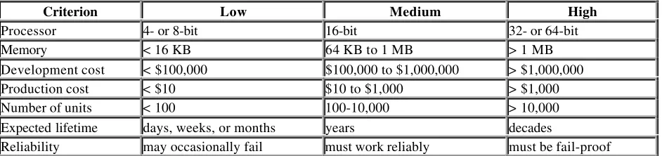
Table 1-1 illustrates the range of possible values for each of the previous design requirements. These are only estimates and should not be taken too seriously. In some cases, two or more of the criteria are linked. For example, increases in processing power could lead to increased production costs. Conversely, we might imagine that the same increase in processing power would have the effect of decreasing the development costs-by reducing the complexity of the hardware and software design. So the values in a particular column do not necessarily go together.
Table 1-1. Common Design Requirements for Embedded Systems
Criterion Low Medium High
Processor 4- or 8-bit 16-bit 32- or 64-bit
Memory < 16 KB 64 KB to 1 MB > 1 MB
Development cost < $100,000 $100,000 to $1,000,000 > $1,000,000
Production cost < $10 $10 to $1,000 > $1,000
Number of units < 100 100-10,000 > 10,000
Expected lifetime days, weeks, or months years decades
Reliability may occasionally fail must work reliably must be fail-proof In order to simultaneously demonstrate the variation from one embedded system to the next and the possible effects of these design requirements on the hardware, I will now take some time to describe three embedded systems in some detail. My goal is to put you in the system designer's shoes for a few moments before beginning to narrow our discussion to embedded software development.
1.2.1 Digital Watch
At the end of the evolutionary path that began with sundials, water clocks, and hourglasses is the digital watch. Among its many features are the presentation of the date and time (usually to the nearest second), the measurement of the length of an event to the nearest hundredth of a second, and the generation of an annoying little sound at the beginning of each hour. As it turns out, these are very simple tasks that do not require very much processing power or memory. In fact, the only reason to employ a processor at all is to support a range of models and features from a single hardware design.
The typical digital watch contains a simple, inexpensive 8-bit processor. Because such small processors cannot address very much memory, this type of processor usually contains its own on-chip ROM. And, if there are sufficient registers available, this application may not require any RAM at all. In fact, all of the electronics-processor, memory, counters and real-time clocks-are likely to be stored in a single chip. The only other hardware elements of the watch are the inputs (buttons) and outputs (LCD and speaker).
The watch designer's goal is to create a reasonably reliable product that has an extraordinarily low production cost. If, after production, some watches are found to keep more reliable time than most, they can be sold under a brand name with a higher markup. Otherwise, a profit can still be made by selling the watch through a discount sales channel. For lower-cost versions, the stopwatch buttons or speaker could be eliminated. This would limit the functionality of the watch but might not even require any software changes. And, of course, the cost of all this development effort may be fairly high, since it will be amortized over hundreds of thousands or even millions of watch sales.
1.2.2 Video Game Player
When you pull the Nintendo-64 or Sony Playstation out from your entertainment center, you are preparing to use an embedded system. In some cases, these machines are more powerful than the comparable generation of personal computers. Yet video game players for the home market are relatively inexpensive compared to personal computers. It is the competing requirements of high processing power and low production cost that keep video game designers awake at night (and their children well-fed).
The companies that produce video game players don't usually care how much it costs to develop the system, so long as the production costs of the resulting product are low-typically around a hundred dollars. They might even encourage their engineers to design custom processors at a development cost of hundreds of thousands of dollars each. So, although there might be a 64-bit processor inside your video game player, it is not necessarily the same type of processor that would be found in a 64-bit personal computer. In all likelihood, the processor is highly specialized for the demands of the video games it is intended to play.
1.2.3 Mars Explorer
In 1976, two unmanned spacecraft arrived on the planet Mars. As part of their mission, they were to collect samples of the Martian surface, analyze the chemical makeup of each, and transmit the results to scientists back on Earth. Those Viking missions are amazing to me. Surrounded by personal computers that must be rebooted almost daily, I find it remarkable that more than 20 years ago a team of scientists and engineers successfully built two computers that survived a journey of 34 million miles and functioned correctly for half a decade. Clearly, reliability was one of the most important requirements for these systems.
What if a memory chip had failed? Or the software had bugs that caused it to crash? Or an electrical connection broke during impact? There is no way to prevent such problems from occurring. So, all of these potential failure points and many others had to be eliminated by adding redundant circuitry or extra functionality: an extra processor here, special memory diagnostics there, a hardware timer to reset the system if the software got stuck, and so on. More recently, NASA launched the Pathfinder mission. Its primary goal was to demonstrate the feasibility of getting to Mars on a budget. Of course, given the advances in technology made since the mid-70s, the designers didn't have to give up too much to accomplish this. They might have reduced the amount of redundancy somewhat, but they still gave Pathfinder more processing power and memory than Viking ever could have. The Mars Pathfinder was actually two embedded systems: a landing craft and a rover. The landing craft had a 32-bit processor and 128 MB of RAM; the rover, on the other hand, had only an 8-bit processor and 512KB. These choices probably reflect the different functional requirements of the two systems. But I'm sure that production cost wasn't much of an issue in either case.
1.3 C: The Least Common Denominator
One of the few constants across all these systems is the use of the C programming language. More than any other, C has become the language of embedded programmers. This has not always been the case, and it will not continue to be so forever. However, at this time, C is the closest thing there is to a standard in the embedded world. In this section I'll explain why C has become so popular and why I have chosen it and its descendent C++ as the primary languages of this book.
Because successful software development is so frequently about selecting the best language for a given project, it is surprising to find that one language has proven itself appropriate for both 8-bit and 64-bit processors; in systems with bytes, kilobytes, and megabytes of memory; and for development teams that consist of from one to a dozen or more people. Yet this is precisely the range of projects in which C has thrived.
Of course, C is not without advantages. It is small and fairly simple to learn, compilers are available for almost every processor in use today, and there is a very large body of experienced C programmers. In addition, C has the benefit of processor-independence, which allows programmers to concentrate on algorithms and applications, rather than on the details of a particular processor architecture. However, many of these advantages apply equally to other high-level languages. So why has C succeeded where so many other languages have largely failed?
Perhaps the greatest strength of C-and the thing that sets it apart from languages like Pascal and FORTRAN-is that it is a very "low-level" high-level language. As we shall see throughout the book, C gives embedded programmers an extraordinary degree of direct hardware control without sacrificing the benefits of high-level languages. The "low-level" nature of C was a clear intention of the language's creators. In fact, Kernighan and Ritchie included the following comment in the opening pages of their book The C Programming Language :
C is a relatively "low level" language. This characterization is not pejorative; it simply
means that C deals with the same sort of objects that most computers do. These may be
combined and moved about with the arithmetic and logical operators implemented by real
machines.
Few popular high-level languages can compete with C in the production of compact, efficient code for almost all processors. And, of these, only C allows programmers to interact with the underlying hardware so easily.
1.3.1 Other Embedded Languages
Of course, C is not the only language used by embedded programmers. At least three other languages-assembly, C++, and Ada-are worth mentioning in greater detail.
In the early days, embedded software was written exclusively in the assembly language of the target processor. This gave programmers complete control of the processor and other hardware, but at a price. Assembly languages have many disadvantages, not the least of which are higher software development costs and a lack of code portability. In addition, finding skilled assembly programmers has become much more difficult in recent years. Assembly is now used primarily as an adjunct to the high-level language, usually only for those small pieces of code that must be extremely efficient or ultra-compact, or cannot be written in any other way.
reduce the efficiency of the executable program. So C++ tends to be most popular with large development teams, where the benefits to developers outweigh the loss of program efficiency.
Ada is also an object-oriented language, though it is substantially different than C++. Ada was originally designed by the U.S. Department of Defense for the development of mission-critical military software. Despite being twice accepted as an international standard (Ada83 and Ada95), it has not gained much of a foothold outside of the defense and aerospace industries. And it is losing ground there in recent years. This is unfortunate because the Ada language has many features that would simplify embedded software development if used instead of C++.
1.3.2 Choosing a Language for the Book
A major question facing the author of a book like this is, which programming languages should be included in the discussion? Attempting to cover too many languages might confuse the reader or detract from more important points. On the other hand, focusing too narrowly could make the discussion unnecessarily academic or (worse for the author and publisher) limit the potential market for the book.
Certainly, C must be the centerpiece of any book about embedded programming-and this book will be no exception. More than half of the sample code is written in C, and the discussion will focus primarily on C-related programming issues. Of course, everything that is said about C programming applies equally to C++. In addition, I will cover those features of C++ that are most useful for embedded software development and use them in the later examples. Assembly language will be discussed in certain limited contexts, but will be avoided whenever possible. In other words, I will mention assembly language only when a particular programming task cannot be accomplished in any other way.
I feel that this mixed treatment of C, C++, and assembly most accurately reflects how embedded software is actually developed today and how it will continue to be developed in the near-term future. I hope that this choice will keep the discussion clear, provide information that is useful to people developing actual systems, and include as large a potential audience as possible.
1.4 A Few Words About Hardware
It is the nature of programming that books about the subject must include examples. Typically, these examples are selected so that they can be easily experimented with by interested readers. That means readers must have access to the very same software development tools and hardware platforms used by the author. Unfortunately, in the case of embedded programming, this is unrealistic. It simply does not make sense to run any of the example programs on the platforms available to most readers-PCs, Macs, and Unix workstations.
Even selecting a standard embedded platform is difficult. As you have already learned, there is no such thing as a "typical" embedded system. Whatever hardware is selected, the majority of readers will not have access to it. But despite this rather significant problem, I do feel it is important to select a reference hardware platform for use in the examples. In so doing, I hope to make the examples consistent and, thus, the entire discussion more clear.
In order to illustrate as many points as possible with a single piece of hardware, I have found it necessary to select a middle-of-the-road platform. This hardware consists of a 16-bit processor (Intel's 80188EB[2] ), a decent amount of
memory (128KB of RAM and 256 KB of ROM), and some common types of inputs, outputs, and peripheral components. The board I've chosen is called the Target188EB and is manufactured and sold by Arcom Control Systems. More information about the Arcom board and instructions for obtaining one can be found in Appendix A.
[2] Intel's 80188EB processor is a special version of the 80186 that has been redesigned for use in embedded systems.
The original 80186 was a successor to the 8086 processor that IBM used in their very first personal computer-the PC/XT. The 80186 was never the basis of any PC because it was passed over (in favor of the 80286) when IBM designed their next model-the PC/AT. Despite that early failure, versions of the 80186 from Intel and AMD have enjoyed tremendous success in embedded systems in recent years.
If you have access to the reference hardware, you will be able to work through the examples in the book exactly as they are presented. Otherwise, you will need to port the example code to an embedded platform that you do have access to. Toward that end, every effort has been made to make the example programs as portable as possible. However, the reader should bear in mind that the hardware in each embedded system is different and that some of the examples might be meaningless on his hardware. For example, it wouldn't make sense to port the Flash memory driver presented in Chapter 6 to a board that had no Flash memory devices.
Chapter 2.
Your First Embedded Program
ACHTUNG! Das machine is nicht fur gefingerpoken und mittengrabben. Ist easy
schnappen der springenwerk, blowenfusen und corkenpoppen mit spitzensparken. Ist
nicht fur gewerken by das dummkopfen. Das rubbernecken sightseeren keepen hands in
das pockets. Relaxen und vatch das blinkenlights!
In this chapter we'll dive right into embedded programming by way of an example. The program we'll look at is similar in spirit to the "Hello, World!" example found in the beginning of most other programming books. As we discuss the code, I'll provide justification for the selection of the particular program and point out the parts of it that are dependent on the target hardware. This chapter contains only the source code for this first program. We'll discuss how to create the executable and actually run it in the two chapters that follow.
2.1 Hello, World!
It seems like every programming book ever written begins with the same example-a program that prints "Hello, World!" on the user's screen. An overused example like this might seem a bit boring. But it does help readers to quickly assess the ease or difficulty with which simple programs can be written in the programming environment at hand. In that sense, "Hello, World!" serves as a useful benchmark of programming languages and computer platforms. Unfortunately, by this measure, embedded systems are among the most difficult computer platforms for programmers to work with. In some embedded systems, it might even be impossible to implement the "Hello, World!" program. And in those systems that are capable of supporting it, the printing of text strings is usually more of an endpoint than a beginning.
You see, the underlying assumption of the "Hello, World!" example is that there is some sort of output device on which strings of characters can be printed. A text window on the user's monitor often serves that purpose. But most embedded systems lack a monitor or analogous output device. And those that do have one typically require a special piece of embedded software, called a display driver, to be implemented first-a rather challenging way to begin one's embedded programming career.
It would be much better to begin with a small, easily implemented, and highly portable embedded program in which there is little room for programming mistakes. After all, the reason my book-writing counterparts continue to use the "Hello, World!" example is that it is a no-brainer to implement. This eliminates one of the variables if the reader's program doesn't work right the first time: it isn't a bug in their code; rather, it is a problem with the development tools or process that they used to create the executable program.
Embedded programmers must be self-reliant. They must always begin each new project with the assumption that nothing works-that all they can rely on is the basic syntax of their programming language. Even the standard library routines might not be available to them. These are the auxiliary functions-like printf and scanf -that most other programmers take for granted. In fact, library routines are often as much a part of the language standard as the basic syntax. However, that part of the standard is more difficult to support across all possible computing platforms and is occasionally ignored by the makers of compilers for embedded systems.
2.2 Das Blinkenlights
Every embedded system that I've encountered in my career has had at least one LED that could be controlled by software. So my substitute for the "Hello, World!" program has been one that blinks an LED at a rate of 1 Hz (one complete on-off cycle per second).[1] Typically, the code required to turn an LED on and off is limited to a few lines
of C or assembly, so there is very little room for programming errors to occur. And because almost all embedded systems have LEDs, the underlying concept is extremely portable.
[1] Of course, the rate of blink is completely arbitrary. But one of the things I like about the 1 Hz rate is that it's easy to
confirm with a stopwatch. Simply start the stopwatch, count off some number of blinks, and see if the number of elapsed seconds is the same as the number of blinks. Need greater accuracy? Simply count off more blinks.
The superstructure of the Blinking LED program is shown below. This part of the program is hardware-independent. However, it relies on the hardware-dependent functions toggleLed and delay to change the state of the LED and handle the timing, respectively.
/********************************************************************** *
* Function: main() *
* Description: Blink the green LED once a second. *
* Notes: This outer loop is hardware-independent. However, * it depends on two hardware-dependent functions. *
* Returns: This routine contains an infinite loop. *
**********************************************************************/ void
main(void) {
while (1) {
toggleLed(LED_GREEN); /* Change the state of the LED. */ delay(500); /* Pause for 500 milliseconds. */ }
} /* main() */
2.2.1 toggleLed
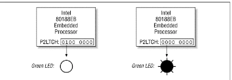
In the case of the Arcom board, there are actually two LEDs: one red and one green. The state of each LED is controlled by a bit in a register called the Port 2 I/O Latch Register (P2LTCH, for short). This register is located within the very same chip as the CPU and takes its name from the fact that it contains the latched state of eight I/O pins found on the exterior of that chip. Collectively, these pins are known as I/O Port 2. And each of the eight bits in the P2LTCH register is associated with the voltage on one of the I/O pins. For example, bit 6 controls the voltage going to the green LED:
#define LED_GREEN 0x40 /* The green LED is controlled by bit 6. */
By modifying this bit, it is possible to change the voltage on the external pin and, thus, the state of the green LED. As shown in Figure 2-1, when bit 6 of the P2LTCH register is 1 the LED is off; when it is the LED is on.
The P2LTCH register is located in a special region of memory called the I/O space, at offset 0xFF5E. Unfortunately, registers within the I/O space of an 80x86 processor can be accessed only by using the assembly language
instructions in and out. The C language has no built-in support for these operations. Its closest replacements are the library routines inport and outport, which are declared in the PC-specific header file dos.h. Ideally, we would just include that header file and call those library routines from our embedded program. However, because they are part of the DOS programmer's library, we'll have to assume the worst: that they won't work on our system. At the very least, we shouldn't rely on them in our very first program.
An implementation of the toggleLed routine that is specific to the Arcom board and does not rely on any library routines is shown below. The actual algorithm is straightforward: read the contents of the P2LTCH register, toggle the bit that controls the LED of interest, and write the new value back into the register. You will notice that although this routine is written in C, the functional part is actually implemented in assembly language. This is a handy technique, known as inline assembly, that separates the programmer from the intricacies of C's function calling and parameter passing conventions but still gives her the full expressive power of assembly language.[2]
[2] Unfortunately, the exact syntax of inline assembly varies from compiler to compiler. In the example, I'm using the
format preferred by the Borland C++ compiler. Borland's inline assembly format is one of the best because it supports references to variables and constants that are defined within the C code.
#define P2LTCH 0xFF5E /* The offset of the P2LTCH register. */ /********************************************************************** *
* Function: toggleLed() *
* Description: Toggle the state of one or both LEDs. *
* Notes: This function is specific to Arcom's Target188EB board. *
* Returns: None defined. *
**********************************************************************/ void
toggleLed(unsigned char ledMask) {
asm {
mov dx, P2LTCH /* Load the address of the register. */ in al, dx /* Read the contents of the register. */ mov ah, ledMask /* Move the ledMask into a register. */ xor al, ah /* Toggle the requested bits. */
out dx, al /* Write the new register contents. */ };
} /* toggleLed() */
2.2.2 delay
/********************************************************************** *
* Function: delay() *
* Description: Busy-wait for the requested number of milliseconds. *
* Notes: The number of decrement-and-test cycles per millisecond * was determined through trial and error. This value is * dependent upon the processor type and speed.
*
* Returns: None defined.
***********************************************************************/ void
delay(unsigned int nMilliseconds) {
#define CYCLES_PER_MS 260 /* Number of decrement-and-test cycles. */
unsigned long nCycles = nMilliseconds * CYCLES_PER_MS;
while (nCycles--);
} /* delay() */
The hardware-specific constant CYCLES_PER_MS represents the number of decrement-and-test cycles (nCycles--!= 0) that the processor can perform in a single millisecond. To determine this number I used trial and error. I made an approximate calculation (I think it came out to around 200), then wrote the remainder of the program, compiled it, and ran it. The LED was indeed blinking but at a rate faster than 1 Hz. So I used my trusty stopwatch to make a series of small changes to CYCLES_PER_MS until the rate of blink was as close to 1 Hz as I cared to test. That's it! That's all there is to the Blinking LED program. The three functions main,toggleLed, and delaydo the whole job. If you want to port this program to some other embedded system, you should read the documentation that came with your hardware, rewrite toggleLed as necessary, and change the value of CYCLES_PER_MS. Of course, we do still need to talk about how to build and execute this program. We'll examine those topics in the next two chapters. But first, I have a little something to say about infinite loops and their role in embedded systems.
2.3 The Role of the Infinite Loop
One of the most fundamental differences between programs developed for embedded systems and those written for other computer platforms is that the embedded programs almost always end with an infinite loop. Typically, this loop surrounds a significant part of the program's functionality-as it does in the Blinking LED program. The infinite loop is necessary because the embedded software's job is never done. It is intended to be run until either the world comes to an end or the board is reset, whichever happens first.
In addition, most embedded systems have only one piece of software running on them. And although the hardware is important, it is not a digital watch or a cellular phone or a microwave oven without that embedded software. If the software stops running, the hardware is rendered useless. So the functional parts of an embedded program are almost always surrounded by an infinite loop that ensures that they will run forever.
This behavior is so common that it's almost not worth mentioning. And I wouldn't, except that I've seen quite a few first-time embedded programmers get confused by this subtle difference. So if your first program appears to run, but instead of blinking the LED simply changes its state once, it could be that you forgot to wrap the calls to toggleLed
Chapter 3.
Compiling, Linking, and Locating
I consider that the golden rule requires that if I like a program I must share it with other
people who like it. Software sellers want to divide the users and conquer them, making
each user agree not to share with others. I refuse to break solidarity with other users in
this way. I cannot in good conscience sign a nondisclosure agreement or a software
license agreement. So that I can continue to use computers without dishonor, I have
decided to put together a sufficient body of free software so that I will be able to get
along without any software that is not free.
-Richard Stallman, Founder of the GNU Project, The GNU Manifesto
In this chapter, we'll examine the steps involved in preparing your software for execution on an embedded system. We'll also discuss the associated development tools and see how to build the Blinking LED program shown in
Chapter 2. But before we get started, I want to make it clear that embedded systems programming is not
substantially different from the programming you've done before. The only thing that has really changed is that each target hardware platform is unique. Unfortunately, that one difference leads to a lot of additional software
complexity, and it's also the reason you'll need to be more aware of the software build process than ever before.
3.1 The Build Process
There are a lot of things that software development tools can do automatically when the target platform is well defined.[1] This automation is possible because the tools can exploit features of the hardware and operating system
on which your program will execute. For example, if all of your programs will be executed on IBM-compatible PCs running DOS, your compiler can automate-and, therefore, hide from your view-certain aspects of the software build process. Embedded software development tools, on the other hand, can rarely make assumptions about the target platform. Instead, the user must provide some of his own knowledge of the system to the tools by giving them more explicit instructions.
[1] Used this way, the term "target platform" is best understood to include not only the hardware but also the operating
system that forms the basic runtime environment for your software. If no operating system is present-as is sometimes the case in an embedded system-the target platform is simply the processor on which your program will be run.
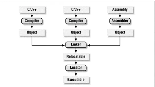
The process of converting the source code representation of your embedded software into an executable binary image involves three distinct steps. First, each of the source files must be compiled or assembled into an object file. Second, all of the object files that result from the first step must be linked together to produce a single object file, called the relocatable program. Finally, physical memory addresses must be assigned to the relative offsets within the relocatable program in a process called relocation. The result of this third step is a file that contains an executable binary image that is ready to be run on the embedded system.
The embedded software development process just described is illustrated in Figure 3-1. In this figure, the three steps are shown from top to bottom, with the tools that perform them shown in boxes that have rounded corners. Each of these development tools takes one or more files as input and produces a single output file. More specific information about these tools and the files they produce is provided in the sections that follow.
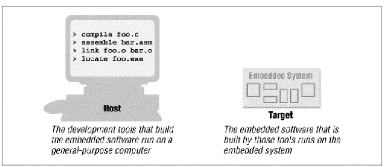
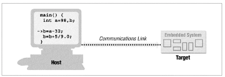
Each of the steps of the embedded software build process is a transformation performed by software running on a general-purpose computer. To distinguish this development computer (usually a PC or Unix workstation) from the target embedded system, it is referred to as the host computer. In other words, the compiler, assembler, linker, and locator are all pieces of software that run on a host computer, rather than on the embedded system itself. Yet, despite the fact that they run on some other computer platform, these tools combine their efforts to produce an executable binary image that will execute properly only on the target embedded system. This split of responsibilities is shown inFigure 3-2.
Figure 3-2. The split between host and target
3.2 Compiling
The job of a compiler is mainly to translate programs written in some human-readable language into an equivalent set of opcodes for a particular processor. In that sense, an assembler is also a compiler (you might call it an "assembly language compiler") but one that performs a much simpler one-to-one translation from one line of human-readable mnemonics to the equivalent opcode. Everything in this section applies equally to compilers and assemblers. Together these tools make up the first step of the embedded software build process.
Of course, each processor has its own unique machine language, so you need to choose a compiler that is capable of producing programs for your specific target processor. In the embedded systems case, this compiler almost always runs on the host computer. It simply doesn't make sense to execute the compiler on the embedded system itself. A compiler such as this-that runs on one computer platform and produces code for another-is called a cross-compiler. The use of a cross-compiler is one of the defining features of embedded software development.
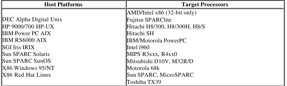
The GNU C/C++ compiler ( gcc ) and assembler (as ) can be configured as either native compilers or cross-compilers. As cross-compilers these tools support an impressive set of host-target combinations. Table 3-1 lists some of the most popular of the supported hosts and targets. Of course, the selections of host platform and target processor are independent; these tools can be configured for any combination.
Table 3-1. Hosts and Targets Supported by the GNU Compiler
Host Platforms Target Processors
DEC Alpha Digital Unix HP 9000/700 HP-UX IBM Power PC AIX IBM RS6000 AIX SGI Iris IRIX Sun SPARC Solaris Sun SPARC SunOS X86 Windows 95/NT X86 Red Hat Linux
AMD/Intel x86 (32-bit only) Fujitsu SPARClite
Hitachi H8/300, H8/300H, H8/S Hitachi SH
IBM/Motorola PowerPC Intel i960
MIPS R3xxx, R4xx0 Mitsubishi D10V, M32R/D Motorola 68k
Sun SPARC, MicroSPARC Toshiba TX39
Regardless of the input language (C/C++, assembly, or any other), the output of the cross-compiler will be an object file. This is a specially formatted binary file that contains the set of instructions and data resulting from the language translation process. Although parts of this file contain executable code, the object file is not intended to be executed directly. In fact, the internal structure of an object file emphasizes the incompleteness of the larger program. The contents of an object file can be thought of as a very large, flexible data structure. The structure of the file is usually defined by a standard format like the Common Object File Format (COFF) or Extended Linker Format (ELF). If you'll be using more than one compiler (i.e., you'll be writing parts of your program in different source languages), you need to make sure that each is capable of producing object files in the same format. Although many compilers (particularly those that run on Unix platforms) support standard object file formats like COFF and ELF (
gcc supports both), there are also some others that produce object files only in proprietary formats. If you're using one of the compilers in the latter group, you might find that you need to buy all of your other development tools from the same vendor.
Most object files begin with a header that describes the sections that follow. Each of these sections contains one or more blocks of code or data that originated within the original source file. However, these blocks have been regrouped by the compiler into related sections. For example, all of the code blocks are collected into a section called text, initialized global variables (and their initial values) into a section called data, and uninitialized global variables into a section called bss.
There is also usually a symbol table somewhere in the object file that contains the names and locations of all the variables and functions referenced within the source file. Parts of this table may be incomplete, however, because not all of the variables and functions are always defined in the same file. These are the symbols that refer to
3.3 Linking
All of the object files resulting from step one must be combined in a special way before the program can be executed. The object files themselves are individually incomplete, most notably in that some of the internal variable and function references have not yet been resolved. The job of the linker is to combine these object files and, in the process, to resolve all of the unresolved symbols.
The output of the linker is a new object file that contains all of the code and data from the input object files and is in the same object file format. It does this by merging the text, data, and bss sections of the input files. So, when the linker is finished executing, all of the machine language code from all of the input object files will be in the text section of the new file, and all of the initialized and uninitialized variables will reside in the new data and bss sections, respectively.
While the linker is in the process of merging the section contents, it is also on the lookout for unresolved symbols. For example, if one object file contains an unresolved reference to a variable named foo and a variable with that same name is declared in one of the other object files, the linker will match them up. The unresolved reference will be replaced with a reference to the actual variable. In other words, if foo is located at offset 14 of the output data section, its entry in the symbol table will now contain that address.
The GNU linker (ld ) runs on all of the same host platforms as the GNU compiler. It is essentially a command-line tool that takes the names of all the object files to be linked together as arguments. For embedded development, a special object file that contains the compiled startup code must also be included within this list. (See Startup Code
later in this chapter.) The GNU linker also has a scripting language that can be used to exercise tighter control over the object file that is output.
Startup Code
One of the things that traditional software development tools do automatically is to insert startup code. Startup code is a small block of assembly language code that prepares the way for the execution of software written in a high-level language. Each high-level language has its own set of expectations about the runtime environment. For example, C and C++ both utilize an implicit stack. Space for the
stack has to be allocated and initialized before software written in either language can be properly executed. That is just one of the responsibilities assigned to startup code for C/C++ programs. Most cross-compilers for embedded systems include an assembly language file called startup.asm, crt0.s (short for C runtime), or something similar. The location and contents of this file are usually described in the documentation supplied with the compiler.
Startup code for C/C++ programs usually consists of the following actions, performed in the order described:
1. Disable all interrupts.
2. Copy any initialized data from ROM to RAM. 3. Zero the uninitialized data area.
4. Allocate space for and initialize the stack. 5. Initialize the processor's stack pointer. 6. Create and initialize the heap.
7. Execute the constructors and initializers for all global variables (C++ only). 8. Enable interrupts.
9. Callmain.
Typically, the startup code will also include a few instructions after the call to main. These instructions will be executed only in the event that the high-level language program exits (i.e., the call to main
returns). Depending on the nature of the embedded system, you might want to use these instructions to halt the processor, reset the entire system, or transfer control to a debugging tool.
If the same symbol is declared in more than one object file, the linker is unable to proceed. It will likely appeal to the programmer-by displaying an error message-and exit. However, if a symbol reference instead remains
unresolved after all of the object files have been merged, the linker will try to resolve the reference on its own. The reference might be to a function that is part of the standard library, so the linker will open each of the libraries described to it on the command line (in the order provided) and examine their symbol tables. If it finds a function with that name, the reference will be resolved by including the associated code and data sections within the output object file.[2]
[2] Beware that I am only talking about static linking here. In non-embedded environments, dynamic linking of libraries
is very common. In that case, the code and data associated with the library routine are not inserted into the program directly.
Unfortunately, the standard library routines often require some changes before they can be used in an embedded program. The problem here is that the standard libraries provided with most software development tool suites arrive only in object form. So you only rarely have access to the library source code to make the necessary changes yourself. Thankfully, a company called Cygnus has created a freeware version of the standard C library for use in embedded systems. This package is called newlib. You need only download the source code for this library from the Cygnus web site, implement a few target-specific functions, and compile the whole lot. The library can then be linked with your embedded software to resolve any previously unresolved standard library calls.
After merging all of the code and data sections and resolving all of the symbol references, the linker produces a special "relocatable" copy of the program. In other words, the program is complete except for one thing: no memory addresses have yet been assigned to the code and data sections within. If you weren't working on an embedded system, you'd be finished building your software now.
But embedded programmers aren't generally finished with the build process at this point. Even if your embedded system includes an operating system, you'll probably still need an absolutely located binary image. In fact, if there is an operating system, the code and data of which it consists are most likely within the relocatable program too. The entire embedded application-including the operating system-is almost always statically linked together and executed as a single binary image.
3.4 Locating
The tool that performs the conversion from relocatable program to executable binary image is called a locator. It takes responsibility for the easiest step of the three. In fact, you will have to do most of the work in this step
yourself, by providing information about the memory on the target board as input to the locator. The locator will use this information to assign physical memory addresses to each of the code and data sections within the relocatable program. It will then produce an output file that contains a binary memory image that can be loaded into the target ROM.
In many cases, the locator is a separate development tool. However, in the case of the GNU tools, this functionality is built right into the linker. Try not to be confused by this one particular implementation. Whether you are writing software for a general-purpose computer or an embedded system, at some point the sections of your relocatable program must have actual addresses assigned to them. In the first case, the operating system does it for you at load time. In the second, you must perform the step with a special tool. This is true even if the locator is a part of the linker, as it is in the case of ld.
The memory information required by the GNU linker can be passed to it in the form of a linker script. Such scripts are sometimes used to control the exact order of the code and data sections within the relocatable program. But here, we want to do more than just control the order; we also want to establish the location of each section in memory. What follows is an example of a linker script for a hypothetical embedded target that has 512 KB each of RAM and ROM:
MEMORY {
ram : ORIGIN = 0x00000, LENGTH = 512K rom : ORIGIN = 0x80000, LENGTH = 512K }
SECTIONS {
data ram : /* Initialized data. */ {
_DataStart = . ; *(.data)
} >rom
bss : /* Uninitialized data. */ {
_BssStart = . ; *(.bss)
_BssEnd = . ; }
_BottomOfHeap = . ; /* The heap starts here. */ _TopOfStack = 0x80000; /* The stack ends here. */
text rom : /* The actual instructions. */ {
*(.text)
} }
This script informs the GNU linker's built-in locator about the memory on the target board and instructs it to locate the data and bss sections in RAM (starting at address 0x00000) and the text section in ROM (starting at 0x80000). However, the initial values of the variables in the data segment will be made a part of the ROM image by the addition of >rom at the end of that section's definition.
All of the names that begin with underscores (_TopOfStack, for example) are variables that can be referenced from within your source code. The linker will use these symbols to resolve references in the input object files. So, for example, there might be a part of the embedded software (usually within the startup code) that copies the initial values of the initialized variables from ROM to the data section in RAM. The start and stop addresses for this operation can be established symbolically, by referring to the integer variables _DataStart and _DataEnd .
The result of this final step of the build process is an absolutely located binary image that can be downloaded to the embedded system or programmed into a read-only memory device. In the previous example, this memory image would be exactly 1 MB in size. However, because the initial values for the initialized data section are stored in ROM, the lower 512 kilobytes of this image will contain only zeros, so only the upper half of this image is significant. You'll see how to download and execute such memory images in the next chapter.
3.5 Building das Blinkenlights
Unfortunately, because we're using the Arcom board as our reference platform, we won't be able to use the GNU tools to build the examples. Instead we'll be using Borland's C++ Compiler and Turbo Assembler. These tools can be run on any DOS or Windows-based PC.[3] If you have an Arcom board to experiment with, this would be a good
time to set it up and install the Borland development tools on your host computer. (See Appendix A for ordering information). I used version 3.1 of the compiler, running on a Windows 95-based PC. However, any version of the Borland tools that can produce code for the 80186 processor will do.
[3] It is interesting to note that Borland's C++ compiler was not specifically designed for use by embedded software
developers. It was instead designed to produce DOS and Windows-based programs for PCs that had 80x86 processors. However, the inclusion of certain command-line options allows us to specify a particular 80x86 processor-the 80186, for example-and, thus, use this tool as a cross-compiler for embedded systems like the Arcom board.
As I have implemented it, the Blinking LED example consists of three source modules: led.c,blink.c, and
startup.asm. The first step in the build process is to compile these two files. The command-line options we'll need are-c for "compile, but don't link," -v for "include symbolic debugging information in the output," -ml for "use the large memory model," and -1 for "the target is an 80186 processor." Here are the actual commands:
bcc -c -v -ml -1 led.c bcc -c -v -ml -1 blink.c
Of course, these commands will work only if the bcc.exe program is in your PATH and the two source files are in the current directory. In other words, you should be in the Chapter2 subdirectory. The result of each of these commands is the creation of an object file that has the same prefix as the .c file and the extension .obj. So if all goes well, there will now be two additional files-led.obj and blink.obj -in the working directory.
theChapter3 subdirectory. To assemble this code into an object file, change to that directory and issue the following command:
tasm /mx startup.asm
The result should be the file startup.obj in that directory. The command that's actually used to link the three object files together is shown here. Beware that the order of the object files on the command line does matter in this case: the startup code must be placed first for proper linkage.
tlink /m /v /s ..\Chapter3\startup.obj led.obj blink.obj, blink.exe, blink.map
As a result of the tlink command, Borland's Turbo Linker will produce two new files: blink.exe and blink.map in the working directory. The first file contains the relocatable program and the second contains a human-readable program map. If you have never seen such a map file before, be sure to take a look at this one before reading on. It provides information similar to the contents of the linker script described earlier. However, these are results and, therefore, include the lengths of the sections and the names and locations of the public symbols found in the relocatable program.
One more tool must be used to make the Blinking LED program executable: a locator. The locating tool we'll be using is provided by Arcom, as part of the SourceVIEW development and debugging package included with the board. Because this tool is designed for this one particular embedded platform, it does not have as many options as a more general locator.[4]
[4] However, being free, it is also a lot cheaper than a more general locator.
In fact, there are just three parameters: the name of the relocatable binary image, the starting address of the ROM (in hexadecimal) and the total size of the destination RAM (in kilobytes):
tcrom blink.exe C000 128
SourceVIEW Borland C ROM Relocator v1.06 Copyright (c) Arcom Control Systems Ltd 1994
Relocating code to ROM segment C000H, data to RAM segment 100H Changing target RAM size to 128 Kbytes
Opening 'blink.exe'... Startup stack at 0102:0402
PSP Program size 550H bytes (2K) Target RAM size 20000H bytes (128K) Target data size 20H bytes (1K) Creating 'blink.rom'...
ROM image size 550H bytes (2K)
Thetcrom locator massages the contents of the relocatable input file-assigning base addresses to each section-and outputs the file blink.rom. This file contains an absolutely located binary image that is ready to be loaded directly into ROM. But rather than load it into the ROM with a device programmer, we'll create a special ASCII version of the binary image that can be downloaded to the ROM over a serial port. For this we will use a utility provided by Arcom, called bin2hex. Here is the syntax of the command:
bin2hex blink.rom /A=1000
Chapter 4.
Downloading and Debugging
I can remember the exact instant when I realized that a large part of my life from then on
was going to be spent in finding mistakes in my own programs.
-Maurice Wilkes, Head of the Computer Laboratory of the University of Cambridge,
1949
Once you have an executable binary image stored as a file on the host computer, you will need a way to download that image to the embedded system and execute it. The executable binary image is usually loaded into a memory device on the target board and executed from there. And if you have the right tools at your disposal, it will be possible to set breakpoints in the program or to observe its execution in less intrusive ways. This chapter describes various techniques for downloading, executing, and debugging embedded software.
4.1 When in ROM ...
One of the most obvious ways to download your embedded software is to load the binary image into a read-only memory device and insert that chip into a socket on the target board. Obviously, the contents of a truly read-only memory device could not be overwritten. However, as you'll see in Chapter 6, embedded systems commonly employ special read-only memory devices that can be progra