Correlation Function and Simplif ied TBA Equations
for XXZ Chain
⋆Minoru TAKAHASHI
Fachbereich C Physik, Bergische Universit¨at Wuppertal, 42097 Wuppertal, Germany E-mail: [email protected]
Received September 27, 2010, in final form December 27, 2010; Published online January 08, 2011
doi:10.3842/SIGMA.2011.004
Abstract. The calculation of the correlation functions of Bethe ansatz solvable models is very difficult problem. Among these solvable models spin 1/2 XXX chain has been investi-gated for a long time. Even for this model only the nearest neighbor and the second neighbor correlations were known. In 1990’s multiple integral formula for the general correlations is derived. But the integration of this formula is also very difficult problem. Recently these integrals are decomposed to products of one dimensional integrals and at zero tempera-ture, zero magnetic field and isotropic case, correlation functions are expressed by log 2 and Riemann’s zeta functions with odd integer argumentζ(3), ζ(5), ζ(7), . . .. We can calculate density sub-matrix of successive seven sites. Entanglement entropy of seven sites is calcu-lated. These methods can be extended to XXZ chain up ton= 4. Correlation functions are expressed by the generalized zeta functions. Several years ago I derived new thermodynamic Bethe ansatz equation for XXZ chain. This is quite different with Yang–Yang type TBA equations and contains only one unknown function. This equation is very useful to get the high temperature expansion. In this paper we get the analytic solution of this equation at ∆ = 0.
Key words: thermodynamic Bethe ansatz equation; correlation function
2010 Mathematics Subject Classification: 16T25; 17B37; 82B23
1
Introduction
We consider the spin 1/2 XXZ chain
H=−J
N
X
l=1
SlxSlx+1+SlySly+1+ ∆
SlzSlz+1−1
4
−2h
N
X
l=1
Slz. (1)
Among the solvable models this model has been investigated for a long time.
It was believed that the exact calculation of correlation function is impossible except the nearest neighbor correlation function. I derived the second neighbor correlation function for
J <0,T = 0, h= 0, ∆ = 1 using the Lieb–Wu solution of one-dimensional Hubbard model [1]. Details are given in Appendix A. In 1990’s multiple integral formula were proposed for h = 0,
T = 0 and recently multiple integral formula was extended toh6= 0,T 6= 0. But the factorization of these multiple integrals to the integrals of lower dimension still remains a difficult problem. I explain the present situation of factorization in Section 2.
Since Yang and Yang proposed the thermodynamic Bethe ansatz (TBA) equation for one dimensional bosons [2], the calculation of free energy becomes important for other solvable models. Yang–Yang type integral equations for (1) were proposed in early 1970’s [3, 4, 5]. In this theory infinite number of unknown functions appeared for |∆| ≥ 1 and finite number of
⋆This paper is a contribution to the Proceedings of the International Workshop “Recent Advances in Quantum
unknowns appear for ∆ = cosπν withν = rational number. The equations change by the value of ∆ and not so convenient for numerical calculations. But some important physical properties at low temperature were investigated using these equations.
Around 1990 the quantum transfer matrix method was applied to this model and numerical results coincide with those of Yang–Yang type equations [6, 7, 8]. In 2001 I proposed a new TBA equation which contains only one unknown function for (1) [9, 10]. This equation is very convenient to do the high-temperature expansions and we get one hundred-th order of high temperature expansion [11]. The traditional cluster expansion method gives up to 22’nd. This method was also applied to the Perk–Schultz model [12].
Unfortunately this equation does not numerically converge at low temperature likeT /|J|<
0.07 because the integrand strongly oscillates. Some other numerical method is necessary. I showed that this equation gives the known exact results in Ising limit (∆ → ∞ and J∆ = finite) [9]. In Section3 I give the analytic solution of this equation for XY case (∆ = 0).
2
Correlation functions of XXZ chain
2.1 Known exact results for J < 0, T = 0, h = 0, ∆ = 1
1. Nearest-neighbor correlator
hSjzSjz+1i= 1 12 −
1
3ln 2 =−0.1477157268. . . (2)
from the ground state energy per site by Hulth´en [13] (1938).
2. Next nearest-neighbor correlator for XXX
hSjzSjz+2i= 1 12 −
4 3ln 2 +
3
4ζ(3) = 0.06067976995. . . , (3)
from the ground state energy of the half-filled Hubbard model by Takahashi [1] (1977). 3. The twisted four-body correlation function
h(Sj×Sj+1)·(Sj+2×Sj+3)i= 1
2ln 2− 3
8ζ(3) =−0.104197748 (4)
from the third derivative of transfer matrix by Muramoto and Takahashi [14] (1999).
2.2 Multiple-integral representations for density matrix
For more general XXZ model with an anisotropy parameter ∆
1. ∆>1,T = 0,h= 0: Vertex operator approachUq( ˆsl(2)) Jimbo, Miki, Miwa, Nakayashiki
[15,16] (1992).
2. −1<∆<1, T = 0,h= 0: qKZ equation Jimbo and Miwa [17] (1996).
3. Rederivation by the quantum inverse scattering method. Generalization to the XXZ model with a magnetic field, T = 0 Kitanine, Maillet, Terras [18] (1998).
4. Integral formula for finite temperature and finite magnetic field G¨ohmann, Kl¨umper, Seel [19] (2004).
Correlation function for successive elementary block
ρn({ǫj, ǫ′j}) = hψ|
n
Q
j=1
Eǫ′j,ǫj
j |ψi
Ej+,+=
is represented by n-fold integral. For example the emptiness formation probability (EFP) for XXX chain at T =h= 0 is
Other arbitrary correlation functions over successive n-sites have similar n-fold integral repre-sentation.
2.3 Boos–Korepin method to evaluate integrals
Here I introduce the details of direct factorization of multiple integrals by Boos and Kore-pin [20,21].
1. Transform the integrand to a certain canonical form without changing the integral value.
2. Perform the integration using the residue theorem.
Example:
Details of transformation are given in Appendix B. In canonical form denominator is
l
Y
k=1
(λ2k−1−λ2k), l≤[n/2].
The n-dimensional integral is decomposed to one and two dimensional integrals. Transform
J1(3)=
Thus second neighbor correlator was rederived from the integral formula. ForP(4) =ρ4++++++++ the integrand is
In 2003, we calculated ρ++−−++−− by Boos–Korepin method and obtained all the correlation func-tions on 4 lattice sites [22]. Especially, the third-neighbor correlator is
The other correlation functions for n= 4 are
From these results we can reproduce the twisted correlation function in (4). In a similar way,P(5) was calculated after very tedious calculations [23]
2.4 Algebraic approach and qKZ relation
Next problem is to calculate hSz
jSjz+4i for XXX model. In principle, it’s possible to calculate other five-dimensional integrals by use of Boos–Korepin method. It, however, will take tremen-dous amount of time.
We propose a different method (“algebraic approach”) and obtain analytical form ofhSz jSjz+4i. This is a generalization of the method by Boos, Korepin, Smirnov (2003) for P(6) [24]. We consider the density matrix ρ of successive n sites of inhomogeneous six vertex model with different spectral parameterzj forj-th site
lim
zi→0
ρǫ′1,...,ǫ′n
n,ǫ1,...,ǫn(z1, z2, . . . , zn) =hE
ǫ′
1 ǫ1 · · ·E
ǫ′
n
ǫni,
(Eǫǫ′)s,s′ =δǫ,sδǫ′,s′, ǫ, ǫ′ =±1.
For n= 1,and 2 we have
ρ+1,+(z1) =ρ−1,−(z1) =
1
2, ρ
−
1,+(z1) =ρ+1,−(z1) = 0, ρ++2,++(z1, z2) =
1 4 +
1
6ω(z1−z2),
ρ+2,−+−(z1, z2) =− 1
6ω(z1−z2), ρ
−+
2,+−(z1, z2) =
1
3ω(z1−z2), with
ω(x)≡ 1
2+ 2
∞ X
k=1
(−1)kk 1−x
2
k2−x2 = 1
2 −2 1−x 2
∞ X
k=0
x2kζa(2k+ 1),
ζa(x)≡
∞ X
n=1
(−1)n−1n−x= 1−21−x
ζ(x), ζa(1) = ln 2,
ω(x+ 1) =−x(x+ 2)
x2−1 ω(x)− 3 2
1
1−x2, ω(−x) =ω(x), ω(±i∞) = 0. The general element of density matrix must satisfy the following algebraic relations.
• Translational invariance
ρǫ′1,...,ǫ′n
n,ǫ1,...,ǫn(z1+x, . . . , zn+x) =ρ
ǫ′
1,...,ǫ′n
n,ǫ1,...,ǫn(z1, . . . , zn).
• Transposition, negating and reverse-order relations
ρǫ′1,...,ǫ′n
n,ǫ1,...,ǫn(z1, . . . , zn) =ρ
ǫ1,...,ǫn
n,ǫ′
1,...,ǫ′n(−z1, . . . ,−zn)
=ρ−ǫ′1,...,−ǫ′n
n,−ǫ1,...,−ǫn(z1, . . . , zn) =ρ
ǫ′
n,...,ǫ′1
n,ǫn,...,ǫ1(−zn, . . . ,−z1). • Intertwining relation
Rǫ′jǫ′j+1
˜
ǫ′
jǫ˜′j+1(zj−zj+1)ρ ...˜ǫ′
j+1,˜ǫ′j...
...ǫj+1,ǫj...(. . . zj+1, zj. . .)
=ρ...ǫ′j,ǫ′j+1...
...˜ǫj,˜ǫj+1...(. . . zj, zj+1. . .)R
˜
ǫj˜ǫj+1
ǫjǫj+1(zj−zj+1),
R++++(z) =R−−−−(z) = 1, R++−−(z) =R−−++(z) = z
z+ 1,
R+−+−(z) =R+−+−(z) = 1
• Reduction relation
ρ+,ǫ′2,...,ǫ′n
n,+,ǫ2,...,ǫn(z1, z2, . . . , zn) +ρ
−,ǫ′
2,...,ǫ′n
n,−,ǫ2,...,ǫn(z1, z2, . . . , zn) =ρ
ǫ′
2,...,ǫ′n
n−1,ǫ2,...,ǫn(z2, . . . , zn).
• First recurrent relation
ρǫ′1,ǫ′2,...,ǫ′n
n,ǫ1,ǫ2,...,ǫn(z+ 1, z, z3, . . . , zn) =−δǫ1,−ǫ2ǫ
′ 1ǫ2ρǫ
′
2,ǫ′3,...,ǫ′n
n−1,−ǫ′
1,ǫ3,...,ǫn(z, z3, . . . , zn),
ρǫ′1,ǫ′2,...,ǫ′n
n,ǫ1,ǫ2,...,ǫn(z−1, z, z3, . . . , zn) =−δǫ′
1,−ǫ′2ǫ1ǫ
′ 2ρ
−ǫ1,ǫ′3,...,ǫ′n
n−1,ǫ2,ǫ3,...,ǫn(z, z3, . . . , zn).
• Second recurrent relation
lim
z1→i∞
ρǫ′1,ǫ′2,...,ǫ′n
n,ǫ1,ǫ2,...,ǫn(z1, z2, . . . , zn) =δǫ1,ǫ′1 1 2ρ
ǫ′
2,...,ǫ′n
n−1,ǫ2,...,ǫn(z2, . . . , zn).
• Identity relations
X
ǫ1,...,ǫn
P
iǫ′i=
P
iǫi
ρǫ′1,...,ǫ′n
n,ǫ1,...,ǫn(z1, . . . , zn) =
X
ǫ′
1,...,ǫ′n
P
iǫ′i=
P
iǫi
ρǫ′1,...,ǫ′n
n,ǫ1,...,ǫn(z1, . . . , zn)
=ρ+n,,...,+,...,++(z1, . . . , zn) =ρ−n,,...,−,...,−−(z1, . . . , zn).
If we assumeρ3 as follows
ρ3+++,+++(z1, z2, z3) = 1
8 +A(z1, z2|z3)ω(z1−z2) +A(z1, z3|z2)ω(z1−z3) +A(z2, z3|z2)ω(z2−z3),
ρ3−,−++++(z1, z2, z3) =ρ2++,++(z2, z3)−ρ3+++,+++(z1, z2, z3),
ρ3−,−++−−(z1, z2, z3) =ρ2−,−++(z1, z2)−ρ3−,−++++(z1, z2, z3), . . . ,
A(z1, z2|z3) =
(z1−z3)(z2−z3)−1 12(z1−z3)(z2−z3)
,
these relations are satisfied. In the homogeneous limitzj →0 this gives the correct correlation
functions of XXX model. In the homogeneous limit each term diverges but we have finite limiting number. Then we can calculate the correlation functions of arbitrary element of density matrix using these algebraic relations, although the calculation become complicated. We have calculated all the inhomogeneous correlation functions up to n≤4 from the multiple integrals and confirmed these relations are fulfilled.
Further we have found the inhomogeneous correlation functions can be represented in terms of ω-function
ρ ǫ′1,...,ǫ′n
n,ǫ1,...,ǫn(z1, . . . , zn) =
n
Y
j=1
δǫj,ǫ′
j
2
+
[n
2]
X
m=1
X
1≤k1<k3<k5<···<k2m−1<n, k2m>k2m−1
Aǫ′1,...,ǫ′n
ǫ1,...,ǫn(k1, . . . , k2m|z1, . . . , zn)ω(zk1 −zk2)· · ·ω(zk2m−1−zk2m),
Aǫ′1,...,ǫ′n
ǫ1,...,ǫn(k1, . . . , k2m|z1, . . . , zn) =
Qǫ′1,...,ǫ′n
ǫ1,...,ǫn(k1, . . . , k2m|z1, . . . , zn)
Q′
i<j(zi−zj)
Denominator is
the same exponent conditions. Unknowns are the coefficients of each terms. Number increases drastically as n, m increases. Algebraic relations give the over complete linear equations. By using mathematica we have unique solution of these equations. By use of algebraic relations, we have calculated all the polynomials forn= 5
Qǫ′1,...,ǫ′5
ǫ1,...,ǫ5(k1, k2|z1, . . . , z5), Q ǫ′
1,...,ǫ′5
ǫ1,...,ǫ5(k1, . . . , k4|z1, . . . , z5). By the memory problem this calculation stopped at n= 6.
Fourth-neighbor correlation function [25]
Using this algebraic method we can calculate all the element of density sub-matrix of successive 6-sites. Longer system is quite difficult because of the memory and computing time problem. We can calculate 6-th neighbor and 7-th neighbor correlations using the generation function method. They are represented by long polynomials of ζa’s. Here we write only numerical results [26]
hSjzSjz+6i= 0.02444673832795890. . . , hSjzSjz+7i=−0.0224982227633722. . . .
2.5 Calculation by continuous dimensions
In a series of papers Boos, Jimbo, Miwa, Smirnov and Takeyama formulated these algebraic calculation by the trace of continuous dimension of auxiliary space [27,28,29,30]
(ρn)ǫǫ11,...,ǫ,...,ǫnn =hvac|(E
ǫ1
ǫ1)1· · ·(E ǫn
hn(ǫ1, . . . , ǫn, ǫn, . . . , ǫ1) = (−1)n
Density sub-matrix in 2n dimensional space is mapped to a vector in 22n dimensional space.
Ωn is an operator in this space. Monodoromy matrix is defined as follows:
L(0)j (λ) =
The trace of any monomial ofI,E,Hand F is a polynomial of dimensiond. One can calculate from the definition (5). For example,
TrdI =d, TrdHH = (d3−d)/3, TrdH = 0.
where the integration path should surround all zj counter-clockwise. In the homogeneous limit
zj →0 Ω becomes
and the calculation becomes very simple. By this formulation we could calculate all the elements of density sub-matrix at n= 7. Calculating the eigenvalues of matrix, we can calculate the von Neumann entropy (entanglement entropy) up to seven sites,
Table 1. von Neumann entropyS(n) of a finite sub-chain of lengthn.
S(1) S(2) S(3) S(4)
1 1.3758573262887466 1.5824933209573855 1.7247050949099274
S(5) S(6) S(7)
1.833704916848315 1.922358833819333 1.997129812895912
2.6 Generalization to XXZ model
In 2003, Kato, Shiroishi, Takahashi, Sakai have generalized the Boos–Korepin method to the XXZ models with an anisotropy parameter |∆| ≤1 for successive three sites [31]. For example
P(n) is represented as follows:
P(n) = (−ν)−n(n2−1)
Here ∆ = cos(πν). Similar integral representations for any arbitrary correlation function for successive three sites were calculated.
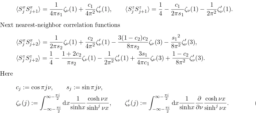
Nearest-neighbor correlation functions
Next nearest-neighbor correlation functions
hSjxSjx+2i= 1
Replacingν →iη/π, we can also get the correlation functions in the massive region ∆ = coshη >
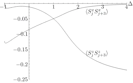
1 [32]. Third neighbor correlations is also expressed by functions ζν and ζν′, although the
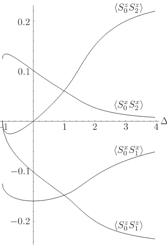
expression becomes more complicated [33]. In Figs. 1 and 2, the nearest neighbor, the second neighbor and the third neighbor correlations are shown as functions of ∆.
3
Simplif ied thermodynamic Bethe ansatz equation
Simplified thermodynamic Bethe ansatz equation at temperature T [9,10] is
Figure 1. The nearest-neighbor and the next nearest neighbor correlation functions for the XXZ chain. We calculated hSz
jSjz+1i,hSjxSjx+1i,hSjzSzj+2iandhSjxSjx+2i.
where
a1(x)≡
θsinθ
2π(coshθx−cosθ). Free energy per site is
f =−Tlnu(0).
In this section we look for analytic solution for XY case ∆ = 0, θ = π/2. For this case equation (7) becomes
u(x)−2 cosh(h/T)−
I π
4 tanh
π
4(x−y)2 cos
J Tsinhπy/2
1
u(y)
dy
2πi = 0.
PuttingX = tanhπx/4,Y = tanhπy/4 and using u(−Y) =u(Y) we have
u(X)−2 cosh(h/T) + 2(1−X2)
I
cos
J
2T
1−Y2 Y
Y
(1−X2Y2)(1−Y2)u(Y)
dY
2πi = 0. (8)
Consider the Fourier transform of following function
g(θ) = 1 2ln
4
cosh2
J
2T sinθ
+ sinh2(h/T)
, aj ≡
Z 2π
0
g(θ) cos(2jθ)dθ 2π.
Assume that
lnu(X) =a0+ 2 ∞ X
j=1
Figure 2. The third-neighbor correlation functions for the XXZ chain.
We can show that this satisfies (8). This series is convergent at |X| ≤1.
lnu(eiθ) + lnu(e−iθ) = 2a0+ 2 ∞ X
j=1
ajcos(2jθ)
= 2g(θ) = ln
4
cosh2
J
2T sinθ
+ sinh2(h/T)
.
Then we have
u(X)u(1/X) = 2 cos
J
2T(X−1/X)
+ 2 + 4 sinh2(h/T). (10)
The function u(X) has zeros at X = ±βj,±, where βj,± = αj,± + q
1 +α2
j,±, and αj,± = 2πT
J (j−
1 2)± 2
hi
J . One can show that |βj,±|>1. u(X) should not have zeros at |X|<1. Then
we have u(X) = const·
∞ Q
j=1
(1−βX22
j,+)(1− X2 β2
j,−
). By the condition u(1) = 2 cosh(h/T) we have infinite product expansion ofu(X)
u(X) = 2 cosh(h/T)
∞ Y
j=1
1−βX22
j,+
1−βX22
j,−
1−β21
j,+
1−β21
j,−
. (11)
From (10) we have
2 cos
J
2T(Y −1/Y)
/u(Y) =u(1/Y)− 2 + 4 sinh2(h/T) /u(Y).
Then we can writeu(X) = 2 cosh(h/T) +v(X2)(1−X2),v(X) =
∞ P
j=0
djXj. Convergence radius
of v(X) is infinite
l.h.s.of (8) =u(X)−2 cosh(h/T) + 1−X2 I
u(1/Y) Y
(1−X2Y2)(1−Y2)
dY πi
= 1−X2
v(X2)−
I
v 1/Y2 1 Y(1−X2Y2)
dY
2πi
= 1−X2 ∞ X
j=0
dj
X2j−
I
1
Y2j+1(1−X2Y2)
dY
2πi
Thus we have proved that (11), (9) satisfies the equation (8). The free energy
−Tlnu(0) =−T a0
coincides with the known result [34].
4
Summary
For J < 0, ∆ = 1, T = h = 0 we obtained the factorized form of density sub-matrix up to
n= 7. The entanglement entropy for seven sites is new result of this paper. Up to six sites we published in [26].
The six-th neighbor and the seven-th neighbor correlations are calculated by the generating function method for J <0, ∆ = 1, T =h= 0 [26].
For arbitrary ∆, T = h = 0 we obtained the factorized form up to n= 4. Correlations are given by two transcendental functions ζν(j) and ζν′(j) with j = 1,3,5, . . . defined by (6). For
correlations ofn≥5 the calculation becomes very tedious and no one has succeeded.
For simplified TBA equation, we obtained the analytic solution for XY limit ∆ = 0. Analytic solution for Ising limit was given in [9].
A
Strong coupling expansion of the Hubbard model
The Hubbard Hamiltonian is written as follows:
H=−tX
<ij>
X
σ
c†iσcjσ+c†jσciσ
+U
Na
X
i=1
c†i↑ci↑c†i↓ci↓.
If we treat the interaction term as main Hamiltonian and hopping therm as perturbation in the half-filled case
H0 =U
X ni↑ni↓,
H1 =−
X
σ
X
i<j
ti,j(c†iσcjσ+c†jσciσ),
the effective Hamiltonian becomes as follows:
Heff =
X
i<j
tijtji
U (σi·σj −1) +U −3
" X
i<j
t4ij(1−σi·σj) +
X
i<k
t2ijt2jk(σi·σk−1)
+ X
i<j<l,i<k,k6=j,l
tijtjktkltli(5(σj ·σk)(σi·σl) + 5(σi·σj)(σk·σl)−5(σj·σk)(σi·σl)
−σi·σj−σj·σk−σk·σl−σl·σi−σi·σk−σj·σl+ 1)
# ,
σi·σj = 4Si·Sj.
For one-dimensional half-filled case the four spin term disappears and the effective Hamiltonian becomes
t2 U
X
i
(4Si·Si+1−1) + t 4
U3
X
i
4(1−4Si·Si+1) + (4Si·Si+2−1) +O
t6 U5
On the other hand exact ground state energy per site is expanded as [35,36]
e=−4|t|
Z ∞
0
J0(ω)J1(ω)dω
ω[1 + exp(2U′ω)]
=−4|t|
"
1 2
2
ln 2U′−1−
1·3 2·4
2 ζ(3)
3
1− 1
22
U′−3+· · ·
#
, (13)
U′ ≡U/(4|t|).
Comparing the first term of (12) and (13), we get nearest neighbor correlation (2). From the second term we get the second neighbor correlation (3).
B
Transformation to canonical form in case of
P
(3)
T3=
(λ1+i)2(λ2+i)λ2λ23
(λ3−λ1−i)(λ3−λ2−i)(λ2−λ1−i)
.
is decomposed to the following three terms,
= i(λ1+i) 2(λ
2+i)λ2λ23 (λ3−λ1−i)(λ2−λ1−i)
+ i(λ1+i) 2(λ
2+i)λ2λ23 (λ3−λ1−i)(λ3−λ2−i)
− i(λ1+i)
2(λ
2+i)λ2λ23 (λ3−λ2−i)(λ2−λ1−i)
.
Using the antisymmetry ofU3(λ1, λ2, λ3) the first and the second terms are simplified as follows:
the first term∼λ21λ2−
(λ1+i)3λ3
λ2−λ1−i
,
the second term∼λ21λ2−
(λ1+i)3(λ3+i)
λ2−λ1−i
.
The third term is transformed as follows
the third term∼ −λ21λ2−i
(λ1+i)3(λ3+i)2
λ2−λ1−i
+i(λ1+i)
3λ2 3
λ2−λ1−i
− i(λ1+i)
3λ3 3
(λ3−λ2−i)(λ2−λ1−i)
.
Then T3 is transformed as follows:
T3∼ −λ2λ23−
i(λ1+i)3λ33 (λ3−λ2−i)(λ2−λ1−i)
.
We should note that the pole at λ3 = 0 and λ1 = −i of U3 is canceled by numerator of the second term. So we can change the integration path λ1→λ1−iand λ3 →λ3+i
T3∼ −λ2λ23−
iλ3
1(λ3+i)3 (λ3−λ2)(λ2−λ1)
.
Using the antisymmetry ofU we have
∼ −λ2λ23− 3λ2
1λ23+ 3iλ1λ23+ 3iλ21λ3−λ23−λ3λ1−λ21
λ2−λ1
.
Thus the denominator is drastically simplified. Using the following relations
λ2 1
λ2−λ1f(λ3)∼
−iλ1+ 13
λ2−λ1 − 1
3(λ1+i)
!
we can reduce the power of numerator,
T3∼ −2λ2λ23+ 1
3 −iλ1−iλ3−2λ1λ3
λ2−λ1
.
Thus we have obtained the canonical form for P(3). The derivation of (14) is as follows:
λ31 λ2−λ1
f(λ3)∼ −
(λ1+i)3
λ2−λ1−i
f(λ3) =
λ32−(λ1+i)3
λ2−λ1−i
− λ
3 2
λ2−λ1−i
f(λ3)
∼
λ3
2−(λ1+i)3
λ2−λ1−i
+(λ2+i) 3
λ2−λ1
f(λ3)∼
λ3
2−(λ1+i)3
λ2−λ1−i
+(λ1+i) 3
λ2−λ1
f(λ3).
Acknowledgements
The author acknowledges to A. Kl¨umper, F. G¨ohmann, H. Boos, J. Sato and M. Shiroishi for stimulating discussions. This work is financially supported by DFG.
References
[1] Takahashi M., Half-filled Hubbard model at low temperature,J. Phys. C10(1977), 1289–1301.
[2] Yang C.N., Yang C.P., Thermodynamics of a one-dimensional system of bosons with repulsive delta-function interaction,J. Math. Phys.10(1969), 1115–1122.
[3] Takahashi M., One-dimensional Heisenberg model at finite temperature, Prog. Theor. Phys. 46 (1971), 401–415.
[4] Gaudin M., Thermodynamics of the Heisenberg–Ising ring for ∆≥1,Phys. Rev. Lett.26(1971), 1301–1304. [5] Takahashi M., Suzuki M., One-dimensional anisotropic Heisenberg model at finite temperatures, Prog.
Theor. Phys.46(1972), 2187–2209.
[6] Koma T., Thermal Bethe-ansatz method for the spin-1/2 XXZ Heisenberg chain, Prog. Theor. Phys. 81 (1989), 783–809.
[7] Takahashi M., Correlation length and free energy ofS= 1/2 XXZ chain in magnetic field,Phys. Rev. B44 (1991), 12382–12394.
[8] Kl¨umper A., Thermodynamics of the anisotropic spin-1/2 Heisenberg chain and related quantum chains, Z. Phys. B91(1993), 507–519,cond-mat/9306019.
[9] Takahashi M., Simplification of thermodynamic Bethe-ansatz equations, in Physics and Combinatrix (Nagoya, 2000), World Sci. Publ., River Edge, NJ, 2001, 299–304,cond-mat/0010486.
[10] Takahashi M., Shiroishi M., Kl¨umper A., Equivalence of TBA and QTM,J. Phys. A: Math. Gen.34(2001), L187–L194,cond-mat/0102027.
[11] Shiroishi M., Takahashi M., Integral equation generates high-temperature expansion of the Heisenberg chain, Phys. Rev. Lett.89(2002), 117201, 4 pages,cond-mat/0205180.
[12] Tsuboi Z., Takahashi M., Nonlinear integral equations for thermodynamics of theUq(sl\(r+ 1)) Perk–Schultz
model,J. Phys. Soc. Japan74(2005), 898–904,cond-mat/0412698.
[13] Hulth´en L., ¨Uber das Austauschproblem eines Kristalles,Ark. Mat. Astron. Fys. A26(1938), 1–105. [14] Muramoto N., Takahashi M., Integrable magnetic model of two chains coupled by four-body interactions,
J. Phys. Soc. Japan68(1999), 2098–2104,cond-mat/9902007.
[15] Jimbo M., Miki K., Miwa T., Nakayashiki A., Correlation functions of the XXZ model for ∆<−1,Phys. Lett. A168(1992), 256–263,hep-th/9205055.
[16] Nakayashiki A., Some integral formulas for the solutions of the sl2 dKZ equation with level-4,Internat. J.
Modern Phys. A9(1994), 5673–5687.
[17] Jimbo M., Miwa T., Quantum KZ equation with|q|= 1 and correlation functions of the XXZ model in the gapless regime,J. Phys. A: Math. Gen.29(1996), 2923–2958,hep-th/9601135.
[19] G¨ohmann F., Kl¨umper A., Seel A., Integral representations for correlation functions of the XXZ chain at finite temperature,J. Phys. A: Math. Gen.37(2004), 7625–7651,hep-th/0405089.
[20] Boos H.E., Korepin V.E., Quantum spin chains and Riemann zeta function with odd arguments,J. Phys. A: Math. Gen.34(2001), 5311–5316,hep-th/0104008.
[21] Boos H.E., Korepin V.E., Evaluation of integrals representing correlations in XXX Heisenberg spin chain, in MathPhys Odyssey (2001),Prog. Math. Phys., Vol. 23, Birkh¨auser Boston, Boston, MA, 2002, 65–108, hep-th/0105144.
[22] Sakai K., Shiroishi M., Nishiyama Y., Takahashi M., Third-neighbor correlators of a one-dimensional spin-1/2 Heisenberg antiferromagnet,Phys. Rev. E67(2003), 065101(R), 4 pages,cond-mat/0302564.
[23] Boos H.E., Korepin V.E., Nishiyama Y., Shiroishi M., Quantum correlations and number theory,J. Phys. A: Math. Gen.35(2002), 4443–4451,cond-mat/0202346.
[24] Boos H.E., Korepin V.E., Smirnov F.A., Emptiness formation probability and quantum Knizhnik– Zamolodchikov equation,Nuclear Phys. B658(2003), 417–439,hep-th/0209246.
[25] Boos H.E., Shiroishi M., Takahashi M., First principle approach to correlation functions of spin-1/2 Heisen-berg chain: fourth-neighbor correlators,Nuclear Phys. B712(2005), 573–599,hep-th/0410039.
[26] Sato J., Shiroishi M., Takahashi M., Correlation functions of the spin-1/2 anti-ferromagnetic Heisenberg chain: exact calculation via the generating function,Nuclear Phys. B729(2005), 441–466,hep-th/0507290. [27] Boos H., Jimbo M., Miwa T., Smirnov F., Takeyama Y., A recursion formula for the correlation functions
of an inhomogeneous XXX model,St. Petersburg Math. J.17(2005), 85–117,hep-th/0405044.
[28] Boos H., Jimbo M., Miwa T., Smirnov F., Takeyama Y., Reduced qKZ equation and correlation functions of the XXZ model,Comm. Math. Phys.261(2006), 245–276,hep-th/0412191.
[29] Boos H., Jimbo M., Miwa T., Smirnov F., Takeyama Y., Traces on the Sklyanin algebra and correlation functions of the eight-vertex model,J. Phys. A: Math. Gen.38(2005), 7629–7659,hep-th/0504072. [30] Boos H., Jimbo M., Miwa T., Smirnov F., Takeyama Y., Density matrix of a finite sub-chain of the
Heisen-berg anti-ferromagnet,Lett. Math. Phys.75(2006), 201–208,hep-th/0506171.
[31] Kato G., Shiroishi M., Takahashi M., Sakai K., Next nearest-neighbor correlation functions of the spin-1/2 XXZ chain at critical region,J. Phys. A: Math. Gen.36(2003), L337–L344,cond-mat/0304475.
[32] Takahashi M., Kato G., Shiroishi M., Next nearest-neighbor correlation functions of the spin-1/2 XXZ chain at massive region,J. Phys. Soc. Japan73(2004), 245–253,cond-mat/0308589.
[33] Kato G., Shiroishi M., Takahashi M. Sakai K., Third-neighbour and other four-point correlation functions of spin-1/2 XXZ chain,J. Phys. A: Math. Gen.37(2004), 5097–5123,cond-mat/0402625.
[34] Takahashi M., Thermodynamics of one-dimensional solvable models, Cambridge University Press, Cam-bridge, 1999.
[35] Lieb E.H., Wu F.Y., Absence of mott transition in an exact solution of the short-range, one-band model in one dimension,Phys. Rev. Lett.20(1968), 1445–1448, Erratum,Phys. Rev. Lett.21(1968), 192.