07350015%2E2014%2E926818

(1)

Full Terms & Conditions of access and use can be found at

http://www.tandfonline.com/action/journalInformation?journalCode=ubes20

Download by: [Universitas Maritim Raja Ali Haji], [UNIVERSITAS MARITIM RAJA ALI HAJI

TANJUNGPINANG, KEPULAUAN RIAU] Date: 11 January 2016, At: 20:57

Journal of Business & Economic Statistics

ISSN: 0735-0015 (Print) 1537-2707 (Online) Journal homepage: http://www.tandfonline.com/loi/ubes20

Comment

Timothy J. Vogelsang

To cite this article: Timothy J. Vogelsang (2014) Comment, Journal of Business & Economic Statistics, 32:3, 334-338, DOI: 10.1080/07350015.2014.926818

To link to this article: http://dx.doi.org/10.1080/07350015.2014.926818

Published online: 28 Jul 2014.

Submit your article to this journal

Article views: 103

View related articles

(2)

334 Journal of Business & Economic Statistics, July 2014

Cox, D. R., and Hinkley, D. V. (1974),Theoretical Statistics, New York: Chap-man and Hall. [330]

Hansen, B. E. (1999), “The Grid Bootstrap and the Autoregressive Model,” Review of Economics and Statistics, 81, 594–607. [332]

McCloskey, A. (2012), “Bonferroni-Based Size-Correction for Nonstandard Testing Problems,” Working paper, Department of Economics, Brown University. Available at http://faculty.wcas.northwestern.edu/∼ate721/ McCloskey_BBCV.pdf. [332]

Mikusheva, A. (2014), “Second Order Expansion of thet-Statistic in AR(1) Models,”Econometric Theory, forthcoming. [332]

M¨uller, U. K. (2007), “A Theory of Robust Long-Run Variance Estimation,” Journal of Econometrics, 141, 1331–1352. [331]

Phillips, P. C. B. (2005), “HAC Estimation by Automated Regression,” Econo-metric Theory, 21, 116–142. [331]

——— (2014), “On Confidence Intervals for Autoregressive Roots and Predic-tive Regression,”Econometrica, 82, 1177–1195. [332]

Phillips, P. C. B., Magdalinos, T., and Giraitis, L. (2010), “Smoothing Local-to-Moderate Unit Root Theory,”Journal of Econometrics, 158, 274–279. [331]

Stock, J. (1991), “Confidence Intervals for the Largest Autoregressive Root in US Macroeconomic Time Series,”Journal of Monetary Economics, 28, 435–459. [332]

Stoica, P., and Moses, R. (2005),Spectral Analysis of Signals, Upper Saddle River, NJ: Pearson Prentice Hall. [331]

Sun, Y. (2006), “Best Quadratic Unbiased Estimators of Integrated Variance in the Presence of Market Microstructure Noise,” Work-ing paper, Department of Economics, UC San Diego. Available at

http://econweb.ucsd.edu/∼yisun/bqu.pdf. [331]

——— (2011), “Autocorrelation Robust Trend Inference With Series Variance Estimator and Testing-optimal Smoothing Parameter,”Journal of Econo-metrics, 164, 345–366. [331]

——— (2013), “A Heteroscedasticity and Autocorrelation Robust F Test Using Orthonormal Series Variance Estimator,”Econometrics Journal, 16, 1–26. [331]

——— (2014a), “Let’s Fix It: Fixed-b Asymptotics versus Small-b Asymptotics in Heteroscedasticity and Autocorrelation Robust Inference,”Journal of Econometrics, 178(3), 659–677. [332]

——— (2014b), “Fixed-Smoothing Asymptotics and Asymptotic F and t Tests in the Presence of Strong Autocorrelation,” Working paper, Department of Economics, UC San Diego. Available athttp://econweb.ucsd.edu/∼yisun/ HAR_strong13_revised.pdf. [331]

Thomson, D. J. (1982), “Spectrum Estimation and Harmonic Analysis,”IEEE Proceedings, 70, 1055–1096. [331]

Comment

Timothy J. V

OGELSANG

Department of Economics, Michigan State University,110 Marshall-Adams Hall, East Lansing, MI 48824 (tjv@msu.edu)

1. INTRODUCTION

Inference in time series settings is complicated by the pos-sibility of strong autocorrelation in the data. In general, some aspect of a time series model is assumed to satisfy stationar-ity and weak dependence assumptions sufficient for laws of large numbers and (functional) central limit theorems to hold. Otherwise, inference is difficult, if not impossible, because in-formation aggregated over time will not be informative. Even if one is willing to allow nonstationarities such as unit root be-havior in the data, various transformations of the data (e.g., first differences) are assumed to satisfy stationarity and weak depen-dence conditions. Time series inference typically performs well when the part of the model that is assumed to satisfy stationar-ity and weak dependence is far from nonstationary boundaries. However, for a given sample size, when the stationary/weak de-pendent part of the model approaches a nonstationary boundary, inference is usually distorted in small samples. The distortions can be quite large. Alternatively, if certain parameter values are close to nonstationary boundaries, then very large sample sizes are needed for accurate inference. Strong autocorrelation is the prototypical case where a model becomes close to a nonstation-ary boundnonstation-ary and accurate inference can be challenging in this case.

For a simple location model and obvious extensions to regres-sions and models estimated by generalized method of moments, M¨uller (2014) proposes a class of tests for single parameters that are robust to strong autocorrelation and maximize a weighted power criterion. As is typical in articles by M¨uller, he takes a systematic and elegant theoretical approach to tackle a difficult econometrics problem. While the test statistic that emerges from

his analysis,Sq, has a complicated form and is far from a priori

obvious, finite sample simulations reported by M¨uller indicate thatSq is very robust to strong autocorrelation and retains

re-spectable power. Comparisons to existing autocorrelation robust tests suggest that theSqtest is a useful addition to the time series

econometrics toolkit.

In this note I make some additional finite sample compar-isons betweenSqand widely usedt-tests based on

nonparamet-ric kernel long run variance estimators. While M¨uller includes some nonparametric kernel-based tests in his comparison group, bandwidth rules are used that tend to pick bandwidths that are too small to effectively control over-rejection problems caused by strong autocorrelation. When autocorrelation is strong, the use of very large bandwidths in conjunction with the fixed-b

critical values of Kiefer and Vogelsang (2005) can lead tot-tests that have similar robustness properties to Sq while retaining

substantial power advantages in some cases. Not surprisingly, the relative performance across tests is sensitive to assump-tions about initial values further illustrating the inherent diffi-culty of carrying out robust inference when autocorrelation is strong.

July 2014, Vol. 32, No. 3 DOI:10.1080/07350015.2014.926818

Color versions of one or more of the figures in the article can be found online atwww.tandfonline.com/r/jbes.

(3)

(a) (b)

(d) (c)

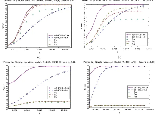
Figure 1. Power ofSqand QS tests. Stationary (I(0)) fixed-bcritical values used for QS tests with no prewhitening.

2. FINITE SAMPLE PROPERTIES

To conserve space, the same notation used by M¨uller is adopted here and definitions of the various test statistics can be found there. The data-generating process is given by

yt =β+ut, t =1,2, . . . , T ,

ut =ρut−1+εt, u0=0, ε0=0,

εt ∼iidN(0,1).

Following M¨uller, consider the following two-sided hypothesis

H0:β=0, H1:β =0.

Results are reported forρ=0.0,0.9,0.98,0.999 using 10,000 replications, andT =200 is used in all cases. The nominal level is 5%. Comparisons are made between (i) three configurations of the new tests:S12,S24, andS48and (ii) the ordinary least squares

(OLS) t-statistic for β based on the quadratic spectral (QS) nonparametric kernel long run variance estimator (Andrews

1991).

The QSt-statistic was considered by M¨uller in his simulation study where it was found that the QS test quickly exhibits large over-rejection problems asρmoves away from 0 and toward 1. Two features of M¨uller’s implementation of the QS statistic pre-clude the possibility of more robust inference asρapproaches 1. First, the bandwidth was chosen using the data-dependent rule proposed by Andrews (1991). The Andrew’s formula tends to pick relatively small bandwidths for the QS kernel even when autocorrelation is strong. Second, standard normal critical val-ues were used to carry out rejections.

Here, I implement the QS test using two bandwidth choices, one small and one very large. Rejections are calculated using the fixed-b critical values proposed by Kiefer and Vogelsang (2005). Referring to formula (4) of M¨uller, ST denotes the

bandwidth of the long run variance estimator. Results are re-ported here for the QS test usingST =8 (small) andST =200

(very large). In the fixed-bframework, these bandwidths map to bandwidth-sample-size ratios,b=ST/T, ofb=8/200=0.04

andb=200/200=1, respectively. The corresponding fixed-b

critical values are 2.115 (b=0.04) and 12.241 (b=1). The use of a very large bandwidth with the fixed-b critical value

(4)

(a) (b)

(d) (c)

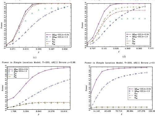
Figure 2. Power ofSqand QS tests. Stationary (I(0)) fixed-bcritical values used for QS tests withAR(1) prewhitening.

can greatly improve the robustness properties of the QS test when autocorrelation is strong relative to the use of a small bandwidth.

Figure 1(a)–1(d) reports power plots of theSqand QS

statis-tics. Power is not size-adjusted and therefore rejections for the case of β=0 represent null rejection probabilities. Because power is not size-adjusted, we can explicitly see the practical trade-off between robustness to over-rejections under the null and power under the alternative.

Whenρ=0 (Figure 1(a)), all tests have empirical null rejec-tions close to 0.05. Power of theSqtests is increasing inq. Power

of the QS tests is high with the small bandwidth (b=0.04) but is substantially lower with the large bandwidth (b=1.0). Whenρ

is close to 1, we see inFigure 1(b)–1(d) that empirical null rejec-tions of the small bandwidth QS test are above 0.05 and substan-tially so whenρ is very close to 1. These large over-rejections were also reported by M¨uller for case where the data-dependent bandwidth was used for QS. In contrast, null rejections for the large bandwidth QS test are much closer to 0.05, and only for

ρ=0.98,0.999 do we begin to see some mild over-rejections. It is important to keep in mind that if the standard normal

crit-ical value had been used instead of the fixed-b critical value, rejections would be substantially above 0.05. While the large bandwidth QS test is relatively robust when autocorrelation is strong, theSq tests are more robust with null rejections very

close to 0.05.

Now consider power. Whenρ=0.9, power of theSq tests

is higher than the large bandwidth QS test for alternatives close to the null but is lower for alternatives far from the null. For the cases with ρ very close to 1, the large band-width QS test has substantially higher power than theSq tests.

This shows that in some cases the remarkable robustness of theSq statistics to strong autocorrelation comes at a high price

with respect to power. If an empirical practitioner is willing to accept a small amount of over-rejection under the null, large gains in power are possible with the large bandwidth QS test.

Suppose one implements the QS tests using a prewhitened version of the nonparametric kernel long run variance esti-mator following Andrews and Monahan (1992).Figure 2(a)–

2(d) reports power plots where QS is implemented with AR(1) prewhitening. As before, results are reported for the small and

(5)

(a) (b)

(d) (c)

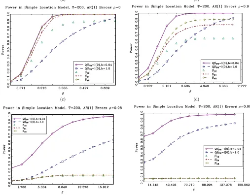
Figure 3. Power of same tests as in Figure 2 but with initial valueu1∼N(0; (1−ρ2)−1) in place ofu1=0.

very large bandwidth QS test with fixed-bcritical values used to compute rejections. Prewhitening only partially reduces the over-rejection problems of the small bandwidth QS test. For the large bandwidth QS test, over-rejections are gone even when

ρ=0.999 and power is not adversely affected.

These simulation results suggest that judicious choice of bandwidth (including potentially very large ones) for the QS statistic and use of fixed-bcritical values can deliver tests that are similarly robust to strong autocorrelation as theSqstatistics

while delivering substantially more power when autocorrela-tion is strong. The challenge is to develop a bandwidth rule that tends to pick small bandwidths when autocorrelation is weak but very large bandwidths when autocorrelation is strong. The data-dependent bandwidth developed by Sun, Phillips, and Jin (2008), which seeks to balance the over-rejection problem with power, does tend to choose larger bandwidths than the Andrews (1991) approach, but the Sun, Phillips, and Jin (2008) band-width rule does not tend to pick bandband-widths large enough to give robustness when autocorrelation is very strong. It would be interesting to see if the Sun, Phillips, and Jin (2008) bandwidth rule could be modified to choose very large bandwidths when

autocorrelation is strong while still choosing small bandwidths when autocorrelation is weak.

Some readers might be wondering why a very large bandwidth is the key to achieving robustness for the QS test when autocor-relation is strong. One way to see this intuitively is to examine the approximate bias of the long run variance estimator given by Equation (4) of M¨uller. Combining results from the traditional spectral analysis literature and the recent fixed-bliterature, one can approximate the bias inω2_k,S

(6)

The first term in the bias,A(b), can be found in Andrews (1991) whereas the second term, B(b), arises because residuals are being used to computeω2

k,ST and was calculated by Hashimzade

et al. (2005) using fixed-btheory.

When a small bandwidth is used, A(b) dominates and the bias is negative (downward) for positively autocorrelated data. As the autocorrelation becomes stronger,A(b) becomes larger in magnitude and the downward bias becomes more pronounced leading to the over-rejections seen in the figures. In contrast, when a large bandwidth is used,A(b) becomes small or even negligible and B(b) dominates the bias. The sign of B(b) is always negative and its magnitude is increasing in the bandwidth (increasing inb). WhereasA(b) is not captured by traditional or fixed-basymptotic theory,B(b) is implicitly captured by the fixed-b limit. Using a large bandwidth minimizes A(b) while maximizingB(b) but fixed-bcritical values correct the impact of B(b) on the t-test, and robustness is achieved. If fixed-b

critical values are not used to correct the large downward bias induced byB(b), substantial over-rejections would be obtained with large bandwidths.

While the QS approach is promising relative to the Sq in

the simple location model, the QS approach does have some drawbacks. Suppose we change the initial condition of{ut}in

the data-generating process to

u1 ∼N(0,(1−ρ2)−1).

Figure 3(a)–3(d) shows power plots for this case. For the cases of ρ =0.0,0.9,0.98 the change in the initial value has little

or no effect on the null rejection probabilities or power of the prewhitened QS statistics or theSqstatistics. However, forρ =

0.999 the large bandwidth QS test now shows nontrivial over-rejections under the null hypothesis. In contrast, theSqstatistics

are unaffected by the change in initial condition. This sensitivity of one class of statistics and the relative insensitivity of another class of statistics to the initial value underscores the conclusion in M¨uller where it is stated that “researchers in the field have to judge which set of regularity conditions makes the most sense for a specific problem.” Robust inference when autocorrelation is strong is not easy.

REFERENCES

Andrews, D. W. K. (1991), “Heteroskedasticity and Autocorrelation Consistent Covariance Matrix Estimation,”Econometrica, 59, 817–854. [335,337] Andrews, D. W. K., and Monahan, J. C. (1992), “An Improved

Heteroskedastic-ity and Autocorrelation Consistent Covariance Matrix Estimator,” Econo-metrica, 60, 953–966. [336]

Hashimzade, N., Kiefer, N. M., and Vogelsang, T. J. (2005), “Moments of HAC Robust Covariance Matrix Estimators Under Fixed-b Asymp-totics,” Working Paper, Department of Economics, Cornell University. [338]

Kiefer, N. M., and Vogelsang, T. J. (2005), “A New Asymptotic Theory for Heteroskedasticity-Autocorrelation Robust Tests,”Econometric Theory, 21, 1130–1164. [334,335]

M¨uller, U. K. (2014), “HAC Corrections for Strongly Autocorrelated Time Series,” Journal of Business and Economic Statistics, 32, 311–322. [334]

Sun, Y., Phillips, P. C. B., and Jin, S. (2008), “Optimal Bandwidth Selection in Heteroskedasticity-Autocorrelation Robust Testing,”Econometrica, 76, 175–194. [337]

Rejoinder

Ulrich K. M ¨

ULLER

Department of Economics, Princeton University, Princeton, NJ, 08544 (umueller@princeton.edu)

I would like to start by expressing my sincere gratitude for the time and effort the reviewers spent on their thoughtful and constructive comments. It is a rare opportunity to have one’s work publicly examined by leading scholars in the field. I will focus on three issues raised by the reviews: the role of the initial condition, applications to predictive regressions, and the relationship to Bayesian inference.

The role of the initial condition under little mean reversion: Vogelsang, Sun, and Cattaneo and Crump all suggest alternative inference procedures for strongly autocorrelated series. Their simulations show that these procedures are substantially more powerful than the Sq tests, especially for distant alternatives

under strong autocorrelation, while coming quite close to con-trolling size. This is surprising, given that the Sq tests are

de-signed to maximize a weighted average power criterion that puts nonnegligible weight on such alternatives.

Recall that theSq tests are constructed to control size under

any stationary AR(1), including values ofρ arbitrarily close to one. Importantly, the initial condition is drawn from the un-conditional distribution. Figure 1 plots four realizations of a mean-zero Gaussian AR(1). For all values ofρclose to one, the

series are almost indistinguishable from a random walk, with the initial condition diverging asρ→1. Yet all of these series are perfectly plausible realizations for a stationarymean-zero

AR(1). Asρ→1, the sample mean is very far from the popula-tion mean relative to the in-sample variapopula-tion. A test that controls size for all values ofρ <1 must not systematically reject the null hypothesis of a zero mean for such series. But the new tests of Sun and Vogelsang, and theτ andτ1/2_{tests of Cattaneo and}

Crump all do so for sufficiently largeρ <1, leading to arbi-trarily large size distortions in this model (see the discussion in Section 6 of the article).

In contrast, theSqtests do not overreject even asρ→1 . The

Sqtests are usefully thought of as joint tests of whether a series

is mean reverting, and whether the long-run mean equals the hypothesized value. The power of any test of this joint problem is clearly bounded above by the power of a test that solely

July 2014, Vol. 32, No. 3 DOI:10.1080/07350015.2014.931769