6. The Returns and Risks from Investing
A
s you continue to prepare yourself to put together and manage a $1 million portfolio, you realize you need to have a very clear understanding of risk and return. After all, as you recall from your introductory finance class, these are the basic parameters of all investing decisions. While you agree that the past is not a sure predictor of the future, it seems reasonable that knowing the history of the returns and risks on the major financial assets will be useful. After all, if stocks in general have never returned more than about 10 percent on average, does it make sense for you to think of earning 15 or 20 percent annually on a regular basis? And what about compounding, supposedly an important part of long-term investing? How much, realistically, can you expect your portfolio to grow over time? Finally, exactly what does it mean to talk about the risk of stocks? How can you put stock risk into perspective? If stocks are really as risky as people say, maybe they should be only a small part of your portfolio.Although math is not your long suit, you realize that it is not unreasonable that a $1 million gift should impose a little burden on you. Therefore, you resolve to get out your financial calculator and go to work on return and risk concepts, knowing that with some basic understanding of the concepts you can take the easy way out and let your computer spreadsheet program do the hard work.
Chapter 6 analyzes the returns and risks from investing. We learn how well investors have done in the past investing in the major financial assets. Investors need a good understanding of the returns and risk that have been experienced to date before attempting to estimate returns and risk, which they must do as they build and hold portfolios for the future.
AFTER READING THIS CHAPTER YOU WILL BE ABLE TO:
Use key terms involved with return and risk, including geometric mean, cumulative wealth index, inflation-adjusted returns, and currency-adjusted returns.
Understand clearly the returns and risk investors have experienced in the past, an important step in estimating future returns and risk.
An Overview
How do investors go about calculating the returns on their securities over time? What about the risk of these securities? Assume you invested an equal amount in each of three stocks over a 5-year period, which has now ended. The five annual returns for stocks 1, 2 and 3 are as follows:
Stock 1 started off with two negative returns but then had three good years. Stock 2's returns are all positive, but quite low. Stock 3 had a 40 percent return in one year and a 17 percent return in another year, but it also suffered three negative returns. Which stock would have produced the largest final wealth for you, and which stock had the lowest risk over this five-year period? Which stock had the lowest compound annual average return over this five-year period? How would you proceed to determine your answers?
Although there is no guarantee that the future will be exactly like the past, a knowledge of historical risk-return relationships is a necessary first step for investors in making investment decisions for the future. Furthermore, there is no reason to assume that relative relationships will differ significantly in the future. If stocks have returned more than bonds, and Treasury bonds more than Treasury bills, over the entire financial history available, there is every reason to assume that such relationships will continue over the long-run future. Therefore, it is very important for investors to understand what has occurred in the past.
Return
In Chapter 1, we learned that the objective of investors is to maximize expected returns subject to constraints, primarily risk. Return is the motivating force in the investment process. It is the reward for undertaking the investment.
Returns from investing are crucial to investors; they are what the game of investments is all about. The measurement of realized (historical) returns is necessary for investors to assess how well they have done or how well investment managers have done on their behalf. Furthermore, the historical return plays a large part in estimating future, unknown returns.
THE TWO COMPONENTS OF ASSET RETURNS
Return on a typical investment consists of two components:
Yield The income component of a security's return
Capital Gain (Loss) The change in price on a security over some period
Yield: The basic component many investors think of when
discussing investing returns is the periodic cash flows (or income) on the investment, either interest (from bonds) or dividends (from stocks). The distinguishing feature of these payments is that the issuer makes the payments in cash to the holder of the asset. Yield measures a security's cash flows relative to some price, such as the purchase price or the current market price.
Capital gain (loss): The second component is the
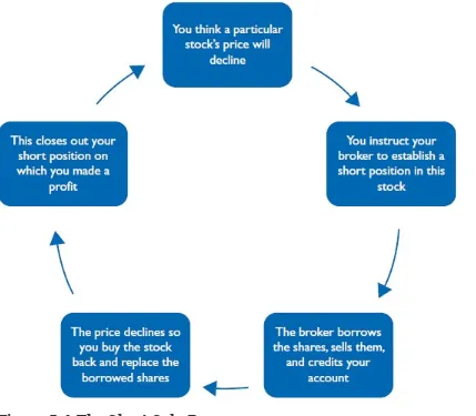
commonly called the capital gain (loss). We will refer to it simply as the price change. In the case of an asset purchased (long position), it is the difference between the purchase price and the price at which the asset can be, or is, sold; for an asset sold first and then bought back (short position), it is the difference between the sale price and the subsequent price at which the short position is closed out. In either case, a gain or a loss can occur.1
Putting the Two Components Together Add these two components together to form the total return:
where the yield component can be 0 or +
the price change component can be 0, +, or −
Example 6-1
A bond purchased at par ($1,000) and held to maturity provides a yield in the form of a stream of cash flows or interest payments, but no price change. A bond purchased for $800 and held to maturity provides both a yield (the interest payments) and a price change, in this case a gain. The purchase of a nondividend-paying stock, such as Apple, that is sold 6 months later produces either a capital gain or a capital loss but no income. A dividend-paying stock, such as Microsoft, produces both a yield component and a price change component (a realized or unrealized capital gain or loss).
Equation 6-1 is a conceptual statement for the total return for any security. Investors' returns from financial assets come only from these two components—an income component (the yield) and/or a price change component, regardless of the asset. Investors sometimes mistakenly focus only on the yield component of their investments, rather than the total return, and mistakenly assume they are achieving acceptable performance when they are not.
Example 6-2
In one recent year a $500,000 portfolio was invested half in stocks and half in bonds. At the end of the year this portfolio had yielded about $19,000 in dividends and interest. However, because of the declining stock market, the value of the portfolio at the end of the year was about $475,000. Therefore, the capital loss exceeded the yield, resulting in a negative total return for that 1-year period.
Total Return (TR) Percentage measure relating all cash flows on a security for a given time period to its purchase price
We now know that a correct returns measure must incorporate the two components of return, yield and price change, keeping in mind that either component could be zero. The total return (TR) for a given holding period is a decimal or percentage number relating all the cash flows received by an investor during any designated time period to the purchase price of the asset calculated as
The periodic cash flows from a bond consists of the interest payments received, and for a stock, the dividends received. For some assets, such as a warrant or a stock that pays no dividends, there is only a price change. Part A of Exhibit 6-1 illustrates the calculation of TR for a bond, a common stock, and a warrant. Although one year is often used for convenience, the TR calculation can be applied to periods of any length.
EXHIBIT 6-1
Examples of Total Return and Price Relative Calculations A. Total Return (TR) Calculations
I. Bond TR
II. Stock TR
Example: 100 shares of DataShield are purchased at $30 per share and sold one year later at $26 per share. A dividend of $2 per share is paid.
III. Warrant TR
where, Ct = any cash payment received by the warrant holder during the period. Because warrants pay no dividends, the only return to an investor from owning a warrant is the change in price during the period.
Example: Assume the purchase of warrants of DataShield at $3 per share, a holding period of six months, and the sale at $3.75 per share.
B. Return Relative Calculations
The return relative for the preceding bond example shown is
The return relative for the stock example is
The return relative for the warrant example is
Calculating Total Returns for the S&P 500 Index Table 6-1 shows the Standard & Poor's (S&P) 500 Stock Composite Index for the years 1926 through 2011 (a total of 86 years because the data start on January 1, 1926). Included in the table are end-of-year values for the index, from which capital gains and losses can be computed, and dividends on the index, which constitute the income component.
Example 6-3
The TRs for each year as shown in Table 6-1 can be calculated as shown in Equation 6-2. As a demonstration of these calculations, the TR for 2010 for the S&P 500 Index was 14.86%, calculated as:2
TR2010 = [1257.64 − 1115.10 + 23.12]/1115.10 = .1486 or 14.86%
In contrast, in 2000 the TR was −9.07 percent, calculated as:
TR2000 = [1320.28 − 1469.25 + 15.69]/1469.25 = −.0907 = −9.07%
Conclusions About Total Return In summary, the total return concept is valuable as a measure of return because it is all-inclusive, measuring the total return per dollar of original investment.
Total Return (TR) is the basic measure of the return earned
by investors on any financial asset for any specified period of time. It can be stated on a decimal or percentage basis.
TR facilitates the comparison of asset returns over a specified period, whether the comparison is of different assets, such as stocks versus bonds, or different securities within the same type, such as several common stocks. Remember that using this concept does not mean that the securities have to be sold and the gains or losses actually realized—that is, the calculation applies to realized or unrealized gains (see Appendix 2-A).
Some Practical Advice
As you analyze and consider common stocks, never forget the important role that dividends have played historically in the TRs shown for large common stocks. For example, for the 85-year period 1926–2010, for the S&P 500 Index, the compound annual average return was 9.6 percent (rounded). Dividends averaged 4 percent, and obviously were an important component of the total return. However, in the 1990s the dividend yield on the major stock indexes continued to decline, and reached levels of about 1.5 percent in 2001 and 2002. Clearly, if all other things remained equal, TRs on the S&P 500 Index would decline relative to the past because of the significant decreases in the dividend yield. Not surprisingly, given the turmoil in the economy, more large companies cut dividends in 2008 than in any year since 2001. At the beginning of 2012, the dividend yield on the S&P 500 Index was approximately 2.1 percent.
What about the importance of dividends for individual stocks? Consider a company with an ordinary product consumed daily around the world, Coca-Cola.
$322,421 at the end of 2011.3 Coca-Cola also paid dividends.
How much impact do you think the reinvested dividends would have on the terminal wealth of this one share at the end of 2011? According to one calculation, that one share would have been worth $9.3 million at the end of 2011! Such is the impact of compounding reinvested dividends over a very long period of time.
RETURN RELATIVE
It is often necessary to measure returns on a slightly different basis than total returns. This is particularly true when calculating either a cumulative wealth index or a geometric mean, both of which are explained below, because negative returns cannot be used in the calculation.
Return Relative (RR) The total return for an investment for a given period stated on the basis of 1.0
The return relative (RR) eliminates negative numbers by
adding 1.0 to the total return. It provides the same information as the TR, but in a different form.
o RR = TR in decimal form + 1.0
o TR in decimal form= RR − 1.0
Example 6-4
A TR of 0.10 for some holding period is equivalent to a return relative of 1.10, and a TR of −9:07, as calculated in Example 6-3 for the year 2000, is equivalent to a return relative of 0.9093.
Equation 6-2 can be modified to calculate return relatives directly by using the price at the end of the holding period in the numerator, rather than the change in price, as in Equation 6-3.
Examples of return relative calculations for the same three assets as the preceding are shown in Part B of Exhibit 6-1.
Example 6-5
The return relative for 2010 for the S&P 500 calculated using equation 6-3 is
(1257.64 + 23.12)/1115.10 = 1.1486
Cumulative Wealth Index Cumulative wealth over time, given an initial wealth and a series of returns on some asset
Return measures such as TRs measure the rate of change in an asset's price or return, and percentage rates of return have multiple uses. Nevertheless, we all understand dollar amounts! Therefore, it is often desirable to measure how one's wealth in dollars changes over time. In other words, we measure the cumulative effect of returns compounding over time given some stated initial investment, which typically is shown as $1 for convenience ($1 is the default value). Note that having calculated ending wealth (cumulative wealth) over some time period on the basis of a $1 initial investment, it is simple enough to multiply by an investor's actual beginning amount invested, such as $10,000 or $22,536 or any other beginning amount.
The Cumulative wealth index, CWIn, is computed as
Example 6-6
Let's calculate cumulative wealth per $1 invested for the 1990s, one of the two greatest decades in the 20th century in which to own common stocks. This will provide you with a perspective on common stock returns at their best. Using the S&P total returns in Table 6-1, and converting them to return relatives, the cumulative wealth index for the decade of the 1990s (the 10-year period 1990– 1999) would be
Thus, $1 (the beginning value arbitrarily chosen) invested at the beginning of 1990 would have been worth $5.23 by the end of 1999. Obviously, any beginning wealth value can be used to calculate cumulative wealth. For example, $10,000 invested under the same conditions would have been worth $52,300 at the end of 1999, and $37,500 invested under the same conditions would have been worth $196,125.
Cumulative wealth is always stated in dollars, and
period of time, given any initial investment. Typically, $1 is used as the initial investment.
Our three returns measures are shown in Figure 6-1.
A Global Perspective
As noted in Chapter 1, international investing offers potential return opportunities and potential reduction in risk through diversification. Based on the historical record, investments in certain foreign markets would have increased investor returns during certain periods of time. For example, in the first decade of the 21st-century European stocks performed much better than U.S. stocks. Dividend yields abroad were about 1 percentage point higher than U.S. dividend yields during that period.
U.S. investors need to understand how the returns on their investment in foreign securities are calculated, and the additional risk they are taking relative to domestic securities. This additional risk may pay off, or penalize them.
Figure 6-1 Three Measures of Return from a Financial Asset
INTERNATIONAL RETURNS AND CURRENCY RISK
Currency Risk (Exchange Rate Risk) The risk of an adverse impact on the return from a foreign investment as a result of movements in currencies
Currency risk (exchange rate risk) is the risk that any change in the value of the investor's home currency relative to the foreign currency involved will be unfavorable; however, like risk in general, currency risk can work in the investor's favor, enhancing the return that would otherwise be received.
How Currency Changes Affect Investors An investment denominated in an appreciating currency relative to the investor's domestic currency will experience a gain from the currency movement, while an investment denominated in a depreciating currency relative to the investor's domestic currency will experience a decrease in the return because of the currency movement. Said differently, when you buy a foreign asset, you sell the home currency to do so, and when you sell the foreign asset, you buy back the home currency. For a U.S. investor,
if the foreign currency strengthens while you hold the
foreign asset, when you sell the asset you will be able to buy back more dollars using the now stronger foreign currency. Your dollar-denominated return will increase.
if the dollar strengthens while you hold the foreign asset, when you sell your asset and convert back to dollars, you will be able to buy back fewer of the now more-expensive dollars, thereby decreasing your dollar-denominated return.
Example 6-7
In one recent year, the Brazilian market was up about 150 percent, but the currency adjustment for U.S. investors was negative (83 percent), leaving a U.S. dollar return for the year of approximately 67 percent instead of 150 percent. On the other hand, the Japanese market enjoyed a 47 percent return, and the currency adjustment was positive, 15 percent, resulting in a U.S. dollar return of approximately 62 percent for the year.
during this period). Assume one share of EurTel at the end of 2002 was €75 (75 Euros). The dollar cost at this time was $1.05 (75) = $78.75. At the end of 2004 the value of one share had risen to €105, an increase of 40 percent for an investor transacting only in Euros. However, the value of the dollar fell sharply during this period, and when the shares of EurTel were sold, the euro proceeds bought back more dollars. The dollar value of one share is now $1.35 (105) = $141.75. The return on this investment, in dollar terms, is (141.75/78.75) − 1.0 = 80 percent.
Table 6-2 Impact of Currency Changes on an Investment in EurTel Stock Denominated in Euros
To calculate directly the return to a U.S. investor from an investment in a foreign country, we can use Equation 6-5. The foreign currency is stated in domestic terms; that is, the amount of domestic currency necessary to purchase one unit of the foreign currency.
Example 6-8
Consider a U.S. investor who invests in WalMex at 40.25 pesos when the value of the peso stated in dollars is $0.10. One year later WalMex is at 52.35 pesos, and the stock did not pay a dividend. The peso is now at $0.093, which means that the dollar appreciated against the peso.
Return relative for WalMex = 52.35/40.25 = 1.3006
In this example, using round numbers, the U.S. investor earned a 30 percent total return denominated in Mexican currency, but only 21 percent denominated in dollars because the peso declined in value against the U.S. dollar. With the strengthening of the dollar, the pesos received when the investor sells WalMex buy fewer U.S. dollars, decreasing the 30 percent return a Mexican investor would earn to only 21 percent for a U.S. investor.
The Dollar and Investors How much difference can currency adjustments make to investors? They can make a substantial difference for selected periods of time.
Example 6-9
Let's consider the impact of the falling dollar on U.S. investors for 1 year, 2007. Canadian stocks earned Canadian investors 10.5 percent, but the gain for U.S. investors was 28.4 percent because of the strengthening of the Canadian dollar against the U.S. dollar. Meanwhile, French investors in a French stock index fund earned only 1.2 percent total return in 2007, while U.S. investors in the same index earned 12.1 percent (as a benchmark, the S&P 500 had a total return of 5.5 percent for 2007).
In 2000 a Euro was worth about $.82. By mid-2008 it was worth roughly $1.56, which means that the value of the dollar declined sharply over this entire period. As the dollar fell, foreign investors owning U.S. stocks suffered from the declining stock market and an unfavorable currency movement. On the other hand, U.S. investors in foreign securities benefited from currency movements. In 2011, despite Greece's sovereign debt crises and other issues about some European countries sovereign debt, as well as concerns about the viability of some financial institutions, the Euro continued to hover around $1.36. This was at least partly a reflection of problems in the United States regarding the national debt and the weak economy. However, in early 2012 the Euro was at $1.27, reflecting the ongoing European crisis.
Investments Intuition
Checking Your Understanding
1. The Cumulative Wealth Index can be calculated for nominal stock returns, but it cannot show the impact of inflation. Agree or disagree, and explain your reasoning.
2. What does it mean to say that when you buy a foreign asset, you are selling the dollar?
3. Is it correct to say that in recent years anti-dollar bets by U.S. investors paid off?
Summary Statistics for Returns
The total return, return relative, and cumulative wealth index are useful measures of return for a specified period of time. Also needed for investment analysis are statistics to describe a series of returns. For example, investing in a particular stock for 10 years or a different stock in each of 10 years could result in 10 TRs, which need to be described by summary statistics. Two such measures used with returns data are described below.
ARITHMETIC MEAN
The best known statistic to most people is the arithmetic mean. Therefore, when someone refers to the mean return they usually are referring to the arithmetic mean unless otherwise specified. The arithmetic mean, customarily designated by the symbol X-bar, of a set of values is calculated as
or the sum of each of the values being considered divided by the total number of values n.
Example 6-10
Based on data from Table 6-1 for the 10 years of the 1990s ending in 1999, the arithmetic mean is calculated in Table 6-3.
GEOMETRIC MEAN
The arithmetic mean return is an appropriate measure of the central tendency of a distribution consisting of returns calculated for a particular time period, such as 10 years. However, when an ending value is the result of compounding over time, the geometric mean, is needed to describe accurately the “true” average rate of return over multiple periods.
Geometric Mean The compound rate of return over time
The geometric mean is defined as the nth root of the product resulting from multiplying a series of return relatives together, as in Equation 6-7.
The geometric mean return measures the compound rate of growth over time. It is important to note that the geometric mean assumes that all cash flows are reinvested in the asset and that those reinvested funds earn the subsequent rates of return available on that asset for some specified period. It reflects the steady growth rate of invested funds over some past period; that is, the uniform rate at which money actually grew over time per period, taking into account all gains and losses.
Example 6-11
Continuing the example from Table 6-3, consisting of the 10 years of data ending in 1999 for the S&P 500, the geometric mean is
Using the Calculator
In Example 6-6, we calculated the CWI for 1990–1999 as 5.23. Knowing this number, we can calculate the geometric mean return for these years by raising 5.23 to yx, taking the 10th root, and subtracting 1.0:
Think of the annual geometric mean as the equal annual return that makes a beginning amount of money grow to a particular ending amount of money.
For example, we saw in Example 6-6 that $1 invested in the S&P 500 Composite Index on January 1, 1990 would have grown to $5.23 by December 31, 1999 (10 years). This is a result of the money compounding at the annual rate of 18 percent. At the end of year 1, the $1 would grow to $1.18; at the end of year 2, the $1.18 would grow to $1.39; at the end of year 3, the $1.39 would grow to $1.64, and so on, until at the end of year 10 the original $1 is worth $5.23. Notice that this geometric average rate of return is lower than the arithmetic average rate of return of 18.76 percent, because it reflects the variability of the returns.
The geometric mean will always be less than the arithmetic
dispersion of the distribution: the greater the dispersion, the greater the spread between the two means.
ARITHMETIC MEAN VERSUS GEOMETRIC MEAN
When should we use the arithmetic mean and when should we use the geometric mean to describe the returns from financial assets? The answer depends on the investor's objective:
The arithmetic mean is a better measure of average
(typical) performance over single periods. It is the best estimate of the expected return for next period.
The geometric mean is a better measure of the change in
wealth over the past (multiple periods). It is typically used by investors to measure the realized compound rate of return at which money grew over a specified period of time.
Example 6-12
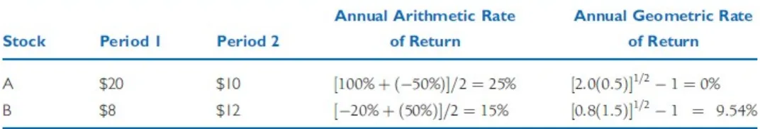
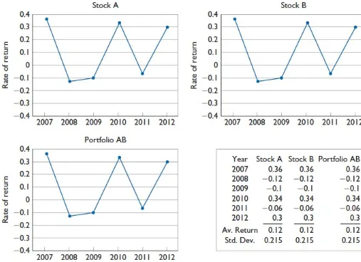
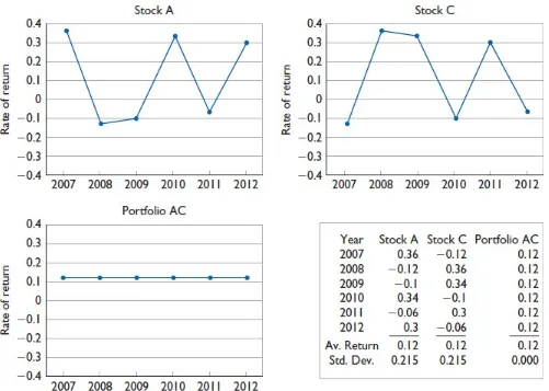
As an illustration of how the arithmetic mean can be misleading in describing returns over multiple periods, consider the data in Table 6-4, which show the movements in price for two stocks over two successive holding periods. Both stocks have a beginning price of $10. Stock A rises to $20 in period 1 and then declines to $10 in period 2. Stock B falls to $8 in period 1 and then rises 50 percent to $12 in period 2. For stock A, the indicated annual average arithmetic rate of change in price is 25 percent [(100% − 50%)/2]. This is clearly not sensible, because the price of stock A at the end of period 2 is $10, the same as the beginning price. The geometric mean calculation gives the correct annual average rate of change in price of 0 percent per year.
For stock B, the arithmetic average of the annual percentage changes in price is 15 percent. However, if the price actually increased 15 percent each period, the ending price in period 2 would be $10 (1.15) (1.15) = $13.23. We know that this is not correct, because the price at the end of period 2 is $12. The annual geometric rate of return, 9.54 percent, produces the correct price at the end of period 2: $10 (1.0954)(1.0954) = $12.
Over multiple periods, such as years, the geometric mean
shows the true average compound rate of growth that actually occurred—that is, the annual average rate at which an invested dollar grew, taking into account the gains and losses over time.
On the other hand, we should use the arithmetic mean to represent the likely or typical performance for a single period. Consider the TR data for the S&P Index for the years 1990–1999 as described earlier. Our best representation of any one year's performance would be the arithmetic mean of 18.76 percent because it was necessary to average this rate of return, given the variability in the yearly numbers, in order to realize an annual compound growth rate of 18 percent after the fact.
Concepts in Action
Using the Geometric Mean to Measure Market Performance
The geometric mean for the S&P 500 Index for the 20th century was 10.35 percent. Thus, $1 invested in this index compounded at an average rate of 10.35 percent every year during the period 1900–1999. What about the first decade of the 21st century (defined as 2000–2009)?
The S&P 500 Index suffered losses for the first 3 years of the decade, followed by positive returns during 2003–2007. 2008 was a disaster, but 2009 showed a very large return. The geometric mean for the first decade is calculated as
INFLATION-ADJUSTED RETURNS
Nominal Return Return in current dollars, with no adjustment for inflation
All of the returns discussed above are nominal returns, based on dollar amounts that do not take inflation into account. Typically, the percentage rates of return we see daily on the news, being paid by financial institutions, or quoted to us by lenders, are nominal rates of return.
Real Returns Nominal (dollar) returns adjusted for inflation
We need to consider the purchasing power of the dollars involved in investing. To capture this dimension, we analyze real returns, or inflation-adjusted returns. When nominal returns are adjusted for inflation, the result is in constant purchasing-power terms. Why is this important to you? What really matters is the purchasing power that your dollars have. It is not simply a case of how many dollars you have, but what those dollars will buy.5
Since 1871, the starting point for reliable data on a broad cross-section of stocks, the United States has had a few periods of deflation, but on average it has experienced mild inflation over a long period of time. Therefore, on average, the purchasing power of the dollar has declined over the long run. We define the rate of inflation or deflation as the percentage change in the CPI.6
Example 6-13
Suppose one of your parents or relatives earned a salary of $35,000 in 1975, and by 2010 his or her salary had increased to $135,000. How much better off is this individual in terms of purchasing power? We can convert the $35,000 in 1975 dollars to 2010 dollars. When we do this, we find that the 1975 salary is worth $141,822 dollars in 2010 dollars. So in terms of purchasing power, this individual has suffered a lost over this long time period.
The Consumer Price Index The Consumer Price Index (CPI) typically is used as the measure of inflation. The compound annual rate of inflation over the period 1926–2010 and over 1926–2011 was 3.00 percent. This means that a basket of consumer goods purchased at the beginning of for $1 would cost approximately $12.34 at year-end 2010. This is calculated as (1.03)85, because there are 85 years from the beginning of 1926 through the end of 2010.7 For 1926–2011, the calculation is
Relation Between Nominal Return and Real Return As an approximation, the nominal return (nr) is equal to the real return (rr) plus the expected rate of inflation (expinf), or
nr ≈ rr + expinf
Reversing this equation, we can approximate the real return as
rr ≈ nr − expinf
To drop the approximation, we can calculate inflation-adjusted returns by dividing 1 + (nominal) total return by 1 + the inflation rate as shown in Equation 6-8.
This equation can be applied to both individual years and average total returns.
Example 6-14
The total return for the S&P 500 Composite in 2004 was 10.87 percent (assuming monthly reinvestment of dividends). The rate of inflation was 3.26 percent Therefore, the real (inflation-adjusted) total return for large common stocks in 2004, as measured by the S&P 500, was
Example 6-15
Consider the period 1926–2011. The geometric mean for the S&P 500 Composite for the entire period was 9.5 percent, and for the CPI, 3.00 percent. Therefore, the real (inflation-adjusted) geometric mean rate of return for large common stocks for the period 1926–2011 was
Checking Your Understanding
5. It is well known that the inflation rate was very low in recent years. Why, then, should investors be concerned with inflation-adjusted returns?
Risk
It is not sensible to talk about investment returns without talking about risk, because investment decisions involve a tradeoff between the two. Investors must constantly be aware of the risk they are assuming, understand how their investment decisions can be impacted, and be prepared for the consequences.
Return and risk are opposite sides of the same coin.
Risk was defined in Chapter 1 as the chance that the actual outcome from an investment will differ from the expected outcome. Specifically, most investors are concerned that the actual outcome will be less than the expected outcome. The more variable the possible outcomes that can occur (i.e., the broader the range of possible outcomes), the greater the risk.
Investors should be willing to purchase a particular asset if the expected return is adequate to compensate for the risk, but they must understand that their expectation about the asset's return may not materialize. If not, the realized return will differ from the expected return. In fact, realized returns on securities show considerable variability—sometimes they are larger than expected, and other times they are smaller than expected, or even negative. Although investors may receive their expected returns on risky securities on a long-run average basis, they often fail to do so on a short-run basis. It is a fact of investing life that realized returns often differ from expected returns.
Investments Intuition
It is important to remember how risk and return go together when investing. An investor cannot reasonably expect larger returns without being willing to assume larger risks. Consider the investor who wishes to avoid any practical risk on a nominal basis. Such an investor can deposit money in an insured savings account, thereby earning a guaranteed return of a known amount. However, this return will be fixed, and the investor cannot earn more than this rate. Although risk is effectively eliminated, the chance of earning a larger return is also removed. To have the opportunity to earn a return larger than the savings account provides, investors must be willing to assume risks—and when they do so, they may gain a larger return, but they may also lose money.
What makes a financial asset risky? In this text we equate risk with variability of returns. One-period rates of return fluctuate over time. Traditionally, investors have talked about several sources of total risk, such as interest rate risk and market risk, which are explained below because these terms are used so widely.
Interest Rate Risk The variability in a security's returns resulting from changes in interest rates Interest Rate Risk The variability in a security's return resulting from changes in the level of interest rates is referred to as interest rate risk. Such changes generally affect securities inversely; that is, other things being equal, security prices move inversely to interest rates.8 Interest rate risk affects bonds more
directly than common stocks, but it affects both and is a very important consideration for most investors.
Market Risk The variability in a security's returns resulting from fluctuations in the aggregate market
Market Risk The variability in returns resulting from fluctuations in the overall market—that is, the aggregate stock market—is referred to as market risk. All securities are exposed to market risk, although it affects primarily common stocks.
Market risk includes a wide range of factors exogenous to securities themselves, including recessions, wars, structural changes in the economy, and changes in consumer preferences. Inflation Risk A factor affecting all securities is purchasing power risk, or the chance that the purchasing power of invested dollars will decline. With uncertain inflation, the real (inflation-adjusted) return involves risk even if the nominal return is safe (e.g., a Treasury bond). This risk is related to interest rate risk, since interest rates generally rise as inflation increases, because lenders demand additional inflation premiums to compensate for the loss of purchasing power.
Financial Risk Financial risk is associated with the use of debt financing by companies. The larger the proportion of assets financed by debt (as opposed to equity), the larger the variability in the returns, other things being equal. Financial risk involves the concept of financial leverage, explained in managerial uncertainty about the time element and the price concession, the greater the liquidity risk. A Treasury bill has little or no liquidity risk, whereas a small OTC stock may have substantial liquidity risk.
Currency Risk (Exchange Rate Risk) All investors who invest internationally in today's increasingly global investment arena face the prospect of uncertainty in the returns after they convert the foreign gains back to their own currency. Investors today must recognize and understand exchange rate risk, which was illustrated earlier in the chapter.
As an example, a U.S. investor who buys a German stock denominated in Euros must ultimately convert the returns from this stock back to dollars. If the exchange rate has moved against the investor, losses from these exchange rate movements can partially or totally negate the original return earned.
Obviously, U.S. investors who invest only in U.S. stocks on U.S. markets do not face this risk, but in today's global environment where investors increasingly consider alternatives from other
need to be considered. The United States has one of the lowest country risks, and other countries can be judged on a relative basis using the United States as a benchmark. In today's world, countries that may require careful attention include Russia, Pakistan, Greece, Portugal, and Mexico.
Measuring Risk
We can easily calculate the average return on stocks over a period of time. Why, then, do we need to know anything else? The answer is that while the average return, however measured, is probably the most important piece of information to an investor, it tells us only the center of the data. It does not tell us anything about the spread of the data.
Risk is often associated with the dispersion in the likely outcomes. Dispersion refers to variability. Risk is assumed to arise out of variability, which is consistent with our definition of risk as the chance that the actual outcome of an investment will differ from the expected outcome. If an asset's return has no variability, in effect it has no risk. Thus, a one-year Treasury bill purchased to yield 10 percent and held to maturity will, in fact, yield (a nominal) 10 percent. No other outcome is possible, barring default by the U.S. government, which is typically not considered a likely possibility.
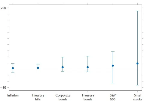
Consider an investor analyzing a series of returns (TRs) for the major types of financial assets over some period of years. Knowing the mean of this series is not enough; the investor also needs to know something about the variability, or dispersion, in the returns. Relative to the other assets, common stocks show the largest variability (dispersion) in returns, with small common stocks showing even greater variability. Corporate bonds have a much smaller variability and therefore a more compact distribution of returns. Of course, Treasury bills are the least risky. The dispersion of annual returns for bills is compact.
Index), and smaller common stocks. (Don't worry about the numbers and the means here—instead, concentrate on the visual range of outcomes for the different asset classes.)
As we can see from Figure 6-2, stocks have a considerably wider range of outcomes than do bonds and bills. Smaller common stocks have a much wider range of outcomes than do large common stocks. Given this variability, investors must be able to measure it as a proxy for risk. They often do so using the standard deviation.
Variance A statistical term measuring dispersion—the standard deviation squared VARIANCE AND STANDARD DEVIATION
Standard Deviation A measure of the dispersion in outcomes around the expected value
Figure 6-2 Graph of Spread in Returns for Major Asset Classes for the Period 1926–2011
SOURCE: Jack W. Wilson and Charles P. Jones.
Knowing the returns from the sample, we can calculate the standard deviation quite easily.
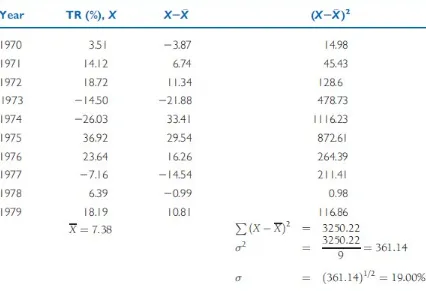
Example 6-16
The standard deviation of the 10 TRs for the decade of the 1970s, 1970–1979, for the Standard & Poor's 500 Index can be calculated as shown in Table 6-5.
In summary, the standard deviation of return measures the total risk of one security or the total risk of a portfolio of securities. The historical standard deviation can be calculated for individual securities or portfolios of securities using TRs for some specified period of time. This ex post value is useful in evaluating the total risk for a particular historical period and in estimating the total risk that is expected to prevail over some future period.
The standard deviation, combined with the normal distribution, can provide some useful information about the dispersion or variation in returns. For a normal distribution, the probability that a particular outcome will be above (or below) a specified value can be determined. With one standard deviation on either side of the arithmetic mean of the distribution, 68.3 percent of the outcomes will be encompassed; that is, there is a 68.3 percent probability that the actual outcome will be within one (plus or minus) standard deviation of the arithmetic mean. The probabilities are 95 and 99 percent that the actual outcome will be within two or three standard deviations, respectively, of the arithmetic mean.
RISK PREMIUMS
Risk Premium That part of a security's return above the risk-free rate of return
A risk premium is the additional return investors expect to receive, or did receive, by taking on increasing amounts of risk. It measures the payoff for taking various types of risk. Such premiums can be calculated between any two classes of securities. For example, a time premium measures the additional compensation for investing in long-term Treasuries versus Treasury bills, and a default premium measures the additional compensation for investing in risky corporate bonds versus riskless Treasury securities.
Equity Risk Premium The difference between stock returns and the risk-free rate
premium measures the difference between stock returns and Treasuries over some past period of time. When we talk about the future, however, we must consider the expected equity risk premium which is, of course, an unknown quantity, since it involves the future.
The equity risk premium affects several important issues and has become an often-discussed topic in Investments. The size of the risk premium is controversial, with varying estimates as to the actual risk premium in the past as well as the prospective risk premium in the future.
Calculating the Equity Risk Premium There are alternative ways to calculate the equity risk premium, involving arithmetic means, geometric means, Treasury bonds, and so forth.
It can be calculated as
1. Equities minus Treasury bills, using the arithmetic mean or the geometric mean
2. Equities minus long-term Treasury bonds, using the arithmetic mean or the geometric mean
Historically the equity risk premium (based on the S&P 500 Index) had a wide range depending upon time period and methodology, but 5–6 percent would be a reasonable average range.
The Expected Equity Risk Premium Obviously, common stock investors care whether the expected risk premium is 5 percent, or 6 percent, because that affects what they will earn on their investment in stocks. Holding interest rates constant, a narrowing of the equity risk premium implies a decline in the rate of return on stocks because the amount earned beyond the risk-free rate is reduced. A number of prominent observers have argued that the equity risk premium in the future is likely to be very different from that of the past, specifically considerably lower.
Checking Your Understanding
7. Why do some market observers expect the equity risk premium in the future to be much lower than it has been in the past?
Realized Returns and Risks From Investing
We can now examine the returns and risks from investing in major financial assets that have occurred in the United States. We also will see how the preceding return and risk measures are typically used in presenting realized return and risk data of interest to virtually all financial market participants.
TOTAL RETURNS AND STANDARD DEVIATIONS FOR THE MAJOR FINANCIAL ASSETS
Table 6-6 shows the average annual geometric and arithmetic returns, as well as standard deviations, for major financial assets for the period 1926–2010 (85 years). Included are both nominal returns and real returns. These data are comparable to those produced and distributed by Ibbotson Associates on a commercial basis. This is an alternative series reconstructed by Jack Wilson and Charles Jones that provides basically the same information (but with a more comprehensive set of S&P 500 companies for the period 1926–1957).10
Source: Jack W. Wilson and Charles P. Jones.
Table 6-6 indicates that large common stocks, as measured by the well-known Standard & Poor's 500 Composite Index, had a geometric mean annual return over this 85-year period of 9.6 percent (rounded). Hence, $1 invested in this market index at the beginning of 1926 would have grown at an average annual compound rate of 9.6 percent over this very long period. In contrast, the arithmetic mean annual return for large stocks was 11.4 percent. The best estimate of the “average” return for stocks in any one year, using only this information, would be 11.4 percent, based on the arithmetic mean, and not the 9.6 percent based on the geometric mean return. The standard deviation for large stocks for 1926–2010 was 19.9 percent.
Example 6-17
Using data with more decimal places than Table 6-6 for 1926–2010 for the S&P 500 Index:
If we know the arithmetic mean of a series of asset returns and the standard deviation of the series, we can approximate the geometric mean for this series. As the standard deviation of the series increases, holding the arithmetic mean constant, the geometric mean decreases.
Although not shown in Table 6-6, smaller common stocks have greater returns and greater risk relative to large common stocks. “Smaller” here means the smallest stocks on the NYSE and not the really small stocks traded on the over-the-counter market. The arithmetic mean for this series is much higher than for the S&P 500 Index, typically 5 or 6 percentage points.11 However,
because of the much larger standard deviation for smaller common stocks, roughly 30 percent, the geometric mean is considerably less than that, typically around 2 percentage points more than the geometric mean for large common stocks (the framework of equation 6-10 explains why there is a large difference between the two means). Small common stocks have by far the largest variability of any of the returns series considered in Table 6-6.
Finally, as we would expect, Treasury bills had the smallest returns of any of the major assets shown in Table 6-6, 3.6 percent, as well as the smallest standard deviation by far.
The deviations for each of the major financial assets in Table 6-6 reflect the dispersion of the returns over the 85-year period covered in the data. The standard deviations clearly show the wide dispersion in the returns from common stocks compared with bonds and Treasury bills. Furthermore, smaller common stocks can logically be expected to be riskier than the S&P 500 stocks, and the standard deviation indicates a much wider dispersion.
CUMULATIVE WEALTH INDEXES
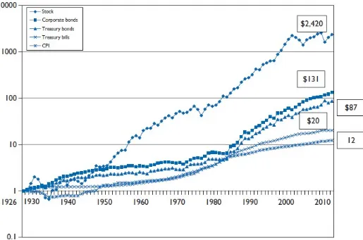
Figure 6-3 Cumulative Wealth for Major Asset Classes and Cumulative Inflation (Amounts are Rounded)
SOURCE: Jack W. Wilson and Charles P. Jones.
As Figure 6-3 shows, the cumulative wealth for stocks, as measured by the S&P 500 Composite Index, completely dominated the returns on corporate bonds over this period— $2,420.46 versus $130.66. Note that we use the geometric mean from Table 6-6 to calculate cumulative ending wealth for each of the series shown in Figure 6-3 by raising (1 + the geometric mean stated as a decimal) to the power represented by the number of periods, which in this case is 85.
Example 6-18
The ending wealth value of $2,420.46 for common stocks in Figure 6-3 is the result of compounding at 9.6 percent for 85 years, or
The large cumulative wealth index value for stocks shown in Figure 6-3 speaks for itself. Remember, however, that the variability of this series is considerably larger than that for bonds or Treasury bills, as shown by the standard deviations in Table 6-6.14
UNDERSTANDING CUMULATIVE WEALTH AS INVESTORS
All of us appreciate dollar totals, and the larger the final wealth accumulated over some period of time, the better. If we fully understand how cumulative wealth comes about from financial assets, in particular stocks, we have a better chance of enhancing that wealth. The cumulative wealth index can be decomposed into the two components of total return, the dividend component and the price change component. To obtain Total Return, we add these two components, but for Cumulative Wealth, we multiply these two components together. Thus,
Conversely, to solve for either of the two components, we divide the CWI by the other component, as in Equation 6-12.
Example 6-19
The CWI for common stocks (S&P 500) for 1926–2010 (85 years) was $2,364.78, based on a geometric mean of 9.57 percent for that period (rounded to 9.6 percent in Table 6-6). The average dividend yield for those 85 years was 3.99 percent. Raising 1.0399 to the 85th power, the cumulative dividend yield, CDY, was $27.82. Therefore, the cumulative price change index for the S&P 500 for that period was $2,364.78/$27.82, or $85.00. This is a compound annual average return of
Note that the annual average geometric mean return relative for common stocks is the product of the corresponding geometric mean return relatives for the two components:
For 1926–2010, an 85-year period,
It is important to understand that for the S&P 500 stocks historically, which many investors hold as an index fund or EFT, dividends played an important role in the overall compound rate of return that was achieved. As we can see, almost 42 percent (3.99%/9.57%) of the total return from large stocks over that long period of time was attributable to dividends.
Dividend yields on the S&P 500 have been low for the past several years, roughly half their historical level. This means that either investors will have to earn more from the price change component of cumulative wealth, or their cumulative wealth will be lower than it was in the past because of the lower dividend yield component.
Compounding and Discounting
Of course, the single most striking feature of Figure 6-3 is the tremendous difference in ending wealth between stocks and bonds. This difference reflects the impact of compounding substantially different mean returns over long periods, which produces almost unbelievable results. The use of compounding points out the importance of this concept and of its complement, discounting. Both are important in investment analysis and are used often. Compounding involves future value resulting from compound interest—earning interest on interest. As we saw, the calculation of wealth indexes involves compounding at the geometric mean return over some historical period.
used extensively in Chapters 10 and 17, and in other chapters as needed.
Summary
Return and risk go together in investments; indeed, these two parameters are the underlying basis of the subject. Everything an investor does, or is concerned with, is tied directly or indirectly to return and risk.
The term return can be used in different ways. It is
important to distinguish between realized (ex post, or historical) return and expected (ex ante, or anticipated) return.
The two components of return are yield and price change (capital gain or loss).
The total return is a decimal or percentage return concept
that can be used to correctly measure the return for any security.
The return relative, which adds 1.0 to the total return, is
used when calculating the geometric mean of a series of returns.
The cumulative wealth index (total return index) is used to
measure the cumulative wealth over time given some initial starting wealth—typically, $1—and a series of returns for some asset.
Return relatives, along with the beginning and ending values of the foreign currency, can be used to convert the return on a foreign investment into a domestic return.
Inflation-adjusted returns can be calculated by dividing 1 +
the nominal return by 1 + the inflation rate as measured by the CPI.
Risk is the other side of the coin: risk and expected return
should always be considered together. An investor cannot reasonably expect to earn large returns without assuming greater risks.
The primary components of risk have traditionally been
categorized into interest rate, market, inflation, business, financial, and liquidity risks. Investors today must also consider exchange rate risk and country risk. Each security has its own sources of risk, which we will discuss when we discuss the security itself.
Historical returns can be described in terms of a frequency
distribution and their variability measured by use of the standard deviation.
The standard deviation provides useful information about
the distribution of returns and aids investors in assessing the possible outcomes of an investment.
Common stocks over the period 1926–2010 had an
annualized geometric mean total return of 9.6 percent, compared to 5.4 percent for long-term Treasury bonds.
Over the period 1920–2010, common stocks had a standard
deviation of returns of approximately 19.9 percent, about two and one-half times that of long-term government and corporate bonds and about six times that of Treasury bills.
Questions
6-1
Distinguish between historical return and expected return.
6-2
6-3 Define the components of total return. Can any of these components be negative?
6-4
Distinguish between TR and holding period return.
6-5
When should the geometric mean return be used to measure returns? Why will it always be less than the arithmetic mean (unless the numbers are identical)?
6-6 When should the arithmetic mean be used in describing stock returns?
6-7
What is the mathematical linkage between the arithmetic mean and the geometric mean for a set of security returns?
6-8 What is an equity risk premium?
6-9
According to Table 6-6, common stocks have generally returned more than bonds. How, then, can they be considered more risky?
6-10
Distinguish between market risk and business risk. How is interest rate risk related to inflation risk?
6-11 Classify the traditional sources of risk as to whether they are general sources of riskor specific sources of risk.
6-12
Explain what is meant by country risk. How would you evaluate the country risk of Canada and Mexico?
6-13 Assume that you purchase a stock on a Japanese market, denominated in yen.During the period you hold the stock, the yen weakens relative to the dollar. Assume you sell at a profit on the Japanese market. How will your return, when converted to dollars, be affected?
6-14 Define risk. How does use of the standard deviation as a measure of risk relate tothis definition of risk?
6-17 Explain how the geometric mean annual average inflation rate can be used tocalculate inflation-adjusted stock returns over the period 1926–2010.
6-18
Explain the two components of the CWI for common stocks. Assume we know one of these two components. How can the other be calculated?
6-19
Common stocks have returned slightly less than twice the compound annual rate of return for corporate bonds. Does this mean that common stocks are about twice as risky as corporates?
6-20 Can cumulative wealth be stated on an inflation-adjusted basis?
6-21
Over the long run, stocks have returned a lot more than bonds, given the compounding effect? Why, then, do investors buy bonds?
6-22 Given the strong performance of stocks over the last 85 years, do you think it ispossible for stocks to show an average negative return over a 10-year period?
6-23
Is there a case to be made for an investor to hold only Treasury bills over a long period of time?
6-24
How can we calculate the returns from holding gold?
6-25 Don't worry too much if your retirement funds earn 5.5% over the next 40 yearsinstead of 6%. It won't affect final wealth very much. Evaluate this claim.
6-26
Suppose someone promises to double your money in 10 years. What rate of return are they implicitly promising you?
6-27 A technical analyst claimed in the popular press to have earned 25% a month for 10years using his technical analysis technique. Is this claim feasible?
6-28
Which alternative would you prefer: (a) 1 percent a month, compounded monthly, or (2) ½ percent a month, compounded semimonthly (24 periods)?
Demonstration Problems
6 -1
The arithmetic mean of the total returns for Extell, 2008–2012:
To calculate the geometric mean in this example, convert the TRs to decimals, and add 1.0, producing return
relatives, RR. The GM is the fifth root of the product of the RRs.
The geometric mean is GM = [(1 + RR1)(1 + RR2)… (1 + RRn)]1/n − 1. Therefore, take the fifth root of the
product
6 -2
The Effects of Reinvesting Returns: The difference in meaning of the arithmetic
and geometric mean, holding Extell stock over the period January 1, 2008 through December 31, 2012 for two different investment strategies, is as follows:
Strategy A—keep a fixed amount (say, $1,000) invested and do not reinvest returns. Strategy B—reinvest returns and allow compounding.
First, take Extell's TRs and convert them to decimal form (r) for Strategy A, and then to (1 +
Using Strategy A, keeping $1,000 invested at the beginning of the year, total returns for the years 2008–2012 were $966, or $193.20 per year average ($966/5), which on a $1,000 investment is $193.20/1000 = 0.1932, or 19.32 percent per year—the same value as the arithmetic mean in Demonstration Problem 6-1 earlier. Using Strategy B, compounding gains and losses, total return was $1,047.46 (the terminal amount $2,047.46 minus the initial $1,000). The average annual rate of return in this situation can be found by taking the root of the terminal/initial amount:
[2047.46/1000]1/5 = (2.0474)1/5 = 1.1541 = (1 + r), r% = 15.41%
which is exactly the set of values we ended up with in Demonstration Problem 6-1 when calculating the geometric mean.
6 -3
Calculating the Standard Deviation: Using the TR values for Extell for the years
2008–2012, we can illustrate the deviation of the values from the mean.
The numerator for the formula for the variance of these Yt values is ∑(Yt-Y)2, which we will call SS
of the squared deviations of the Yt around the mean. Algebraically, there is a simpler alternative formula.
The variance is the “average” squared deviation from the mean:
The standard deviation is the square root of the variance:
σ = (σ2)1/2 = (1284.532)1/2 = 35.84%
The standard deviation is in the same units of measurement as the original observations, as is the arithmetic mean.
6 -4
Calculation of Cumulative Wealth Index and Geometric Mean: By using the
geometric mean annual average rate of return for a particular financial asset, the cumulative wealth index can be found by converting the TR on a geometric mean basis to a return relative, and raising this return relative to the power representing the number of years involved. Consider the geometric mean of 12.47 percent for small common stocks for the period 1926–2007. The cumulative wealth index, using a starting index value of $1, is (note the 82 periods):
$1(1.1247)82 = $15,311.19
Conversely, if we know the cumulative wealth index value, we can solve for the geometric mean by taking
the nth root and subtracting out 1.0.
($15,311.19)1/82 − 1.0 = 1.1247 − 1.0 = .1247 or 12.47%
6 -5
Calculation of Inflation-Adjusted Returns: Knowing the geometric mean for
inflation for some time period, we can add 1.0 and raise it to the nth power. We then divide the cumulative wealth index on a nominal basis by the ending value for inflation to obtain inflation-adjusted returns. For example, given a cumulative wealth index of $2,364.78 for common stocks for 1926–2010, and a geometric mean inflation rate of 3.00 percent, the inflation-adjusted cumulative wealth index for this 85-year period is calculated as
$2364.78/(1.03)85 = $2364.78/12.336 = $191.70
6 -6
Analyzing the Components of a Cumulative Wealth Index: Assume that we know
that for the period 1926–2010 the yield component for common stocks was 3.99 percent, and that the cumulative wealth index was $2,364.78. The cumulative wealth index value for the yield component was
(1.0399)85 = 27.82
The cumulative wealth index value for the price change component was $2,364.78/27.82 = 85.00
The geometric mean annual average rate of return for the price change component for common stocks was
(85.00)1/85 = 1.0537
The geometric mean for common stocks is linked to its components by the following: 1.0399(1.0537) = 1.0957; 1.0957 − 1.0 = .0957 or 9.57%
The cumulative wealth index can be found by multiplying together the individual component cumulative wealth indexes:
Calculate the TR and the return relative for the following assets:
1. A preferred stock bought for $70 per share, held 1 year during which $5 per share dividends are collected, and sold for $63
2. A warrant bought for $11 and sold three months later for $13
3. A 12 percent bond bought for $870, held 2 years during which interest is collected, and sold for $930
6-2
does this change when 2003 is included?
6-3
Calculate the index value for the S&P 500 (Table 6-1) assuming a $1 investment at the beginning of 1980 and extending through the end of 1989. Using only these index values, calculate the geometric mean for these years.
6-4
Assume that one of your relatives, on your behalf, invested $100,000 in a trust holding S&P 500 stocks at the beginning of 1926. Using the data in
determine the value of this trust at the end of 2010.
6-5 Now assume that your relative had invested $100,000 in a trust holding “smallstocks” at the beginning of 1926. Determine the value of this trust at the end of 2010.
6-6
What if your relative had invested $100,000 in a trust holding long-term Treasury bonds at the beginning of 1926. Determine the value of this trust at the end of 2010.
6-7
Finally, what if this relative had invested $100,000 in a trust holding Treasury bills at the beginning of 1926. Determine the value of this trust by the end of 2010.
6-8
Calculate cumulative wealth for corporate bonds for the period 1926–2010, using a geometric mean of 5.9 percent (85-year period).
6-9
Given a cumulative wealth index for Treasury bills of $20.21 for the period 1926– 2010, calculate the geometric mean.
6-10 Given an inflation rate of 3 percent over the period 1926–2010 (geometric meanannual average), calculate the inflation-adjusted cumulative wealth index for corporate bonds as of year-end 2010.
6-11
Given a geometric mean inflation rate of 3 percent, determine how long it would take to cut the purchasing power of money in half using the rule of 72.
6-12
If a basket of consumer goods cost $1 at the beginning of 1926 and $12.34 at the end of 2010, calculate the geometric mean rate of inflation over this period.
6-13
Assume that over the period 1926–2010 the yield index component of common stocks had a geometric mean annual average of 3.99 percent. Calculate the cumulative wealth index for this component as of year-end 2010. Using this value, calculate the cumulative wealth index for the price change component of common stocks using information in Figure 6-3.
6-14
Assume that Treasury bonds continued to have a geometric mean as shown in