I.-Chen Wu, Member, IEEE, Der-Johng Sun, Lung-Ping Chen, Kan-Yueh Chen, Ching-Hua Kuo, Hao-Hua Kang, and Hung-Hsuan Lin - An Efficient Approach to Solving Nonograms

An Ef

_fi

cient Approach to Solving Nonograms

I.-Chen Wu

, Member, IEEE

, Der-Johng Sun, Lung-Ping Chen, Kan-Yueh Chen, Ching-Hua Kuo,

Hao-Hua Kang, and Hung-Hsuan Lin

Abstract—_{A nonogram puzzle is played on a rectangular grid}

of pixels with clues given in the form of row and column con-straints. The aim of solving a nonogram puzzle, an NP-complete problem, is to paint all the pixels of the grid in black and white while satisfying these constraints. This paper proposes an efficient approach to solving nonogram puzzles. We propose a fast dynamic programming (DP) method for line solving, whose time complexity in the worst case is only, where the grid size is and is the average number of integers in one constraint, always smaller than . In contrast, the time complexity for the best line-solving method in the past is . We also propose some fully probing (FP) methods to solve more pixels before running backtracking. Our FP methods can solve more pixels than the method proposed by Batenburg and Kosters (before backtracking), while having a time complexity that is smaller than theirs by a factor of . Most importantly, these FP methods provide useful guidance in choosing the next promising pixel to guess during backtracking. The proposed methods are incorporated into a fast nonogram solver, named LalaFrogKK. The program outperformed all the programs collected in webpbn.com, and also won both nonogram tournaments that were held at the 2011 Conference on Tech-nologies and Applications of Artificial Intelligence (TAAI 2011, Taiwan). We expect that the proposed FP methods can also be applied to solving other puzzles efficiently.

Index Terms—_{Backtracking, fully probing (FP), nonogram,}

NP-completeness, painted by number, puzzles.

I. INTRODUCTION

N

ONOGRAM [19], also known asHanjie,Paint by Num-bers, orGriddlers, is one of the popular logic puzzles in-vented by a Japanese graphics editor named Non Ishida in 1988. In 1990, the U.K. newspaperThe Sunday Telegraphstarted pub-lishing nonogram puzzles on a weekly basis [14].

A nonogram puzzle is played on a given rectangular grid of cells, alternatively referred to as pixels, with clues given in the form of row and column constraints. The aim of solving a nonogram puzzle is to paint all the pixels of the grid in black and white while satisfying these given constraints. A nonogram puzzle is illustrated in Fig. 1(a), where in an 8 8 grid row constraints are given in the rightmost column and column con-straints are given in the bottom row. In this paper, symbol “ ”

Manuscript received September 28, 2012; revised January 09, 2013 and Feb-ruary 19, 2013; accepted FebFeb-ruary 27, 2013. Date of publication March 08, 2013; date of current version September 11, 2013. This work was supported by the National Science Council of the Republic of China (Taiwan) under Con-tracts NSC 99-2221-E-009-102-MY3 and NSC 99-2221-E-009-104-MY3.

I.-C. Wu, D.-J. Sun, K.-Y. Chen, C.-H. Kuo, H.-H. Kang, and H.-H. Lin are with the Department of Computer Science, National Chiao-Tung University, Hsinchu 30050, Taiwan (e-mail icwu@csie.nctu.edu.tw).

L.-P. Chen is with the Department of Computer Science and Information En-gineering, Tung-Hai University, Taichung 40704, Taiwan.

Color versions of one or more of thefigures in this paper are available online at http://ieeexplore.ieee.org.

Digital Object Identifier 10.1109/TCIAIG.2013.2251884

Fig. 1. (a) A nonogram puzzle given in [21] and (b) its solution.

stands for a pixel that is to be painted, and “ ” and “ ” stand for a pixel painted in black and white, respectively. The integers in these constraints are used to indicate the lengths of black seg-ments in the solution shown in Fig. 1(b). A black segment is a set of maximally consecutive black pixels in a row (or a column). For example, the constraints of the third row, 1 3, indicate that the row in the solution has two, and only two, black segments where the length of the_first segment (leftmost) is 1 and that of the second segment is 3. It is not required to have unique so-lutions for nonogram puzzles, but most puzzles published for human players normally have unique solutions.

Solving a nonogram puzzle ef_ficiently is challenging, espe-cially those that are large. Ueda and Nagao showed [17] that the general problem of determining whether a nonogram puzzle has a solution is NP-complete.

In the past, several researchers studied how to solve nono-gram puzzles by translating them into other problems. Bosch [5] translated a nonogram problem into an integer linear pro-gramming (IPL) problem and solved it accordingly. Faase [8] translated it into an exact cover problem and we can then use Knuth’s dancing-links method [9] to solve it. Unfortunately, the sizes of the translated problems are usually too large to solve ef_ficiently. Batenburg [1] modi_fied an evolutionary algorithm for discrete tomography (DT) to solve nonogram puzzles, while Wiggers [18] used a genetic algorithm. However, both methods do not guarantee exact solutions.

Many researchers have been engaged in the study of solving nonogram puzzles ef_ficiently. In [24], Yuet al. proposed an algorithm to solve nonogram puzzles based on speci_fic log-ical rules, using backtracking to solve undetermined cells and logical rules to improve the search ef_ficiently. These logical rules are mainly used to help line painting (either for rows or columns), with the goal of painting as many pixels in each line as possible. Some simpler line painting methods were also men-tioned in [13] and [15]. However, these methods are not

anteed to solve lines. In this paper, line solving means painting the maximum number of pixels for given lines.

For line solving, Batenburg and Kosters [2] proposed a dy-namic programming (DP) method instead of speci_fic logical rules. In general, this method paints more pixels than those in [13], [15], and [24], and runs much faster. Assume that the grid size of a given puzzle is and the average number of in-tegers in one constraint is , which is smaller than . In the worst case, the time complexity for solving each line using the DP method is estimated to be . Furthermore, Batenburg and Kosters [2] also used a 2-Satis_fiability (2-SAT) method to help paint more pixels in whole grids (before backtracking), and the time complexity for the method was , estimated in Section III-D. In addition to the above research, many nono-gram solvers have been designed, collected, and published in [21], and nonogram-generating algorithms have been discussed in [2] and [3].

In this paper, based on the research in [2], we propose a faster DP method for line solving, whose time complexity in the worst case is only, which improves that in [2] by . In addi-tion, we propose three fully probing (FP) methods, named FP1, FP2, and FP3, to paint more pixels before backtracking. The time complexities for both FP1 and FP2 (before backtracking) are , while that for FP3 is . In the case that the FP methods alone cannot paint the entire grid, backtracking will be used to_finish the process. Most importantly, the FP methods also provide backtracking with useful information as guidance in choosing the next pixel to guess.

The proposed methods were also incorporated into a nono-gram solver, named LALAFROGKK, which won both nonogram tournaments that were held at the 2011 Conference on Tech-nologies and Applications of Arti_ficial Intelligence (TAAI 2011, Taiwan) [10]. The program also outperformed all the programs collected in [21].

In the rest of this paper, Section II describes our methods for line solving and propagation. Section III proposes three FP methods to solve more pixels before backtracking. Section IV describes backtracking. Experiments are presented in Section V, and concluding remarks are given in Section VI.

II. LINESOLVING ANDPROPAGATION

In this section,_first, we specify the de_finitions and notations in Section II-A. Then, we describe our methods for line solving in Section II-B. Propagation of line solving in the whole grid is given in Section II-C.

A. Definitions and Notation

As described in Section I, a nonogram puzzle is given initially with a rectangular grid, a sequence of row descriptions for row constraints, and a sequence of column descriptions for column constraints. Each is again a sequence of integers , where is the number of integers in the sequence. Similarly, each is a sequence of integers , where is the number of integers in the sequence. The goal of solving the puzzle is to paint all the

pixels of the grid in black or white such that the following conditions hold.

1) Each row (column ) in the grid includes black segments (de_fined in Section I).

2) Each integer indicates the length of the th black segment from the left in row (from the top in column ). For simplicity of discussion, consider a line, instead of a row or a column. Let a line be represented by a string , where denotes the length of the line (or the number of pixels in the line), and each indicates the color of the th pixel in the line. The substring

is a segment of the line, where . Let be a symbol 0 (or 1), if the th pixel in the line is painted in white (or black). Segment , where , is a black segment, if all are 1’s, and both and , if they exist, are 0’s. Following the notation in [2] for the string representation, let be the_finite alphabet , and be the set of all the strings over of length . For simplicity, let be the set of all the strings over of all lengths. For simplicity of discussion, a pattern for strings is expressed in a regular expression notation. For example, both 0100111 and 001100 match pattern .

As de_fined above, each line (either row or column) is given by a description, say . Line

is said to be consistent with , if is the number of black seg-ments in the line, and each is the length of the th black seg-ment (starting from ). More speci_fically, given description , line is consistent with if matches the following pattern:

Let denote segment of length . Let denote the concatenation of 0 and . The above can be rewritten as follows for line consistency. Given is consistent with if

matches the following pattern:

Among all the strings that match the pattern, the minimal string

length is .

When a line is partially painted, some pixels in the line may not be painted yet, since the colors of these pixels are still un-known. In line , let be the symbol if the th pixel has not yet been painted. Following the notation in [2] for the string representation, let be the_finite alphabet, and be the set of all the strings over of length . For line , if some , the th pixel will need to be changed to either 0 or 1, but notvice versa. For line , no further changes are required.

String is said to be an assignment

of another string , if the following three conditions hold: 1) if is 0, then is 0; 2) if is 1, then is 1; and 3) if is , then is one of 0, 1, or . Let denote the assignment relation between and . For example, 0100, 0110, and are assignments of , that is,

, and . Following [2], an assignment of is also called a_fix of , if . For simplicity, let denote and .

consistent with . For example, is_fixable with respect to since_fix (for ) is consistent with . In addition, string is said to match pattern , if there exists_fix of such that matches . For example, matches .

String is said to be partially_fixable to string

with respect to description , if is an assignment of and is_fixable with respect to . For simplicity, the relation is

denoted by . For example, we have

, and .

B. Line Solving

This section studies methods to paint a partially painted line with respect to a description. We investigate two problems,_fi xa-bility and line solving, as described in Sections II-B1 and II-B2, and then give a discussion in Section II-B3.

1) Fixability: The _fixability problem is as follows:

Given string and description

, verify whether is _fixable with respect to . As mentioned in Section II-A, is con-sistent with if matches the following pattern: . For simplicity, let us as-sume that is already 0 in the rest of this section. If is not 0, we simply add one 0 at the beginning of .

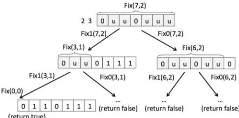
For this_fixability problem, we propose a DP method, which is more ef_ficient than the one in [2]. Our method is to build a recurrence for all and as follows. Let denote string , and denote description . Given and veri_fies whether is_fixable with respect to , as shown in Proposition 1. In addition, let indicate whether string is_fixable with respect to in the case that matches 0, and, similarly, let indicate_fixability for the case where matches 1. An example is illustrated in Fig. 2. The recurrences for

are formulated in detail as follows:

true if and

false if and

otherwise

if false otherwise

if and

matches

false otherwise.

Proposition 1: For the above recurrences, is true if is_fixable with respect to , and false, otherwise. The solution to the_fixability problem, therefore, is the value of . To derive this value, we use the typical DP method [7] by calculating a table with size , where the table is a 2-D array of data returned from for all . Since it takes only constant time to calculate each , the time complexity for evaluating is clearly . In con-trast, the time complexity given in [2] is . In practice, the above method can be further improved by checking whether

Fig. 2. Fix0(7, 2) for a string with respect to .

in all . If not, return false immedi-ately. This is because the minimal length of strings_fixable with respect to is , as mentioned in Section II-A.

2) Line Solving: This section describes our line-solving method. Before discussing it, we de_fine the equivalence of two strings with respect to a description in De_finition 1.

Definition 1: Let string . Let be the set of all fixes , where . For another string

and are called to be equivalent with respect to , denoted by

, if .

Furthermore, a painting and the maximal painting of a string are de_fined in De_finition 2.

Definition 2: String is called a painting of with respect to , denoted by , if and . Painting is called the maximal painting of with respect to , denoted by , if the following condition holds: for all , where

, we have .

The above de_finitions are illustrated by an example with string and description . Clearly, the _fix set is . All the strings, , and , are paintings from with respect to , since their_fix sets with respect to are the same as . Among these paintings, is the maximal

painting of , that is, .

The line-solving problem is as follows: Given string and description , _find the maximal painting of , that is, . The maximal painting can be derived from , the intersection of all possible_fixes, as follows. Given a set of _fixes is de_fined to be string satisfying the following properties for each :

1) , if the th pixel is 0 for all strings ; 2) , if the th pixel is 1 for all strings ;

3) , if the th pixel is 0 for some string and 1 for some other string .

Proposition 2: From the above de_finitions, given string and , the following properties are satis_fied:

1) is the maximal painting of with respect to ;

2) if , then ;

3) if , then ;

4) if , then (from the

Proposition 2 shows some properties. The _first property is that is the maximal painting of with respect to . From the previous example, and .

We have , and

, which is the maximal painting of . The next three properties are illustrated by an example with an additional

, where . The_fix sets and

are and , respectively, satisfying . Both maximal paintings are, respectively,

and , satisfying .

For the line-solving problem, we also use a DP method, mod-i_fied from the one used for the computation of to_find the maximal painting of a given with re-spect to a given . Similarly, let denote string , and denote description . Given and , where is true (that is, is fixable with respect to ), the recurrence for all and _finds the maximal painting of with respect to , as shown in Lemma 1. The recurrences are described in the equation at the bottom of the page.

Lemma 1: For the above recurrences, if is true,

returns .

Proof: In the case that , it is trivial that

simply returns null string . Note that if and , then is false, and, thus, is not called.

In the case that returns ,

which then derives from and

, respectively, for cases and .

Re-currence returns if

is true, and returns

, if is true.

Since is true from the assumption of this lemma and from Section II-A, one of the three conditions holds: 1) is true and

is false; 2) is false and is true; and 3) both and are true.

Assume that the _first condition holds. Then, all _fixes

in are also in , that is,

. Hence, simply

returns , which returns .

Sim-ilarly, assuming that the second condition holds, simply returns .

Assume that the third condition holds. Let and

de-note and , respectively.

Ob-viously, . Hence,

de-rives by merging and , which

are returned by and , respectively. Let and denote and , respectively. and are merged using the above function . Let and be

and , respectively. Function merges each pair of pixels pairwise by . First, the th pixel of the returning string is 0 if both and are 0, for the following reason. Since , the th pixels for all strings in must be 0. Similarly, since , the th pixels for all strings in must be 0. Thus, th pixels in all strings must be 0 as well. Therefore, the th pixel of the returning string is 0. For the same reason, in function , the th pixel of the returning string is 1 if both and are 1.

For all the other cases for both and , function

returns for the th pixel for the following reason. The rest of the cases can be classi_fied into the following two subcases: 1) one of and is 0 and the other is 1; and 2) at least one of and is . In the_first subcase, since one is for 0 and the other for 1, the pixel must be for property 3 of maximal painting. In the second subcase, since one is already , indicating that some is for 0 and some other for 1, the pixel must be as well.

Let us illustrate this by using the above example: Given

and , use to derive

, that is, . In this example, both and are true, and both

and return

and , respectively. Thus,

merges both, and returns .

Thus, returns .

For deriving the maximal painting , we also use DP to calculate a table with size , where the table is a 2-D array of data returned from for all . Since it takes or time to merge two strings, the time complexity for evaluating is . In fact, the time complexity can be further reduced to theoretically, as explained in the Appendix. For this reason, the time complexity will be used in the analysis in the rest of this paper.

3) Discussion: In this section, two issues are discussed. The first issue to consider is the case of general multicolor

nono-if otherwise

if and not if not and otherwise

where if

if

grams, where has more than two elements. In these kinds of puzzles, the descriptions should also include the colors of each segment. A general method for is to use , instead of , where is the color of the last segment. indicates whether string is_fixable with respect to in the case where the last character matches in the description. In this way, the time complexity is still the same.

Another issue is of practical design. Since the line lengths (widths or heights) of most nonogram puzzles are normally below or around 30, we can use bit vectors to implement lines. For example, we use two bits to indicate a pixel, bits 01 for 0, 10 for 1, and 11 for , and use a 64-bit word to represent a line with no more than 32 pixels. Thus, the merging operation simply performs one bitwise-or operation on two 64-bit words. In this sense, the time complexity can also be viewed as .

C. Propagation

This section applies the algorithm of line solving, described in Section II-B, to solving nonogram puzzle . Let the given nonogram puzzle have a rectangular grid of pixels, and denote the pixel at row and column . Let the puzzle have rows, denoted by , where each represents , and columns, denoted

by , where each represents .

The propagation problem involves repeatedly painting pixels with values of into 0 or 1 by applying line solving to all rows and all columns, until none of the pixels in the grid can be painted. In this section, we design an ef_ficient routine, named PROPAGATE, to solve the propagation problem as follows.

procedurePROPAGATE

1. ; // is a set of updated pixels 2. Put all rows and columns of into

3. while do

4. Retrieve one line from

5. Let the line be ,that is, row ; // for simplicity of discussion

6. if then CONFLICT;

return 7.

8. Let be the newly painted pixels of

9. For each pixel in ,put its column into the list ,if not in yet

10. ; // collect all painted cells in this propagate

In PROPAGATE, denotes a list of lines (columns or rows) in that are to be solved. For simplicity of analysis, let

. Initially, the queue contains all lines ( rows and columns). During each iteration (between lines 4 and 10 in the pseudocode above), retrieve from only one line, say row ,

without loss of generality. Then, and are the string and the description of the row, respectively. Then, use to check (in line 6) whether a con_flict is detected in the row. Assume that is false. Then, the row is not_fixable for the puzzle, which implies a con_flict with the hints of the puzzle in the cur-rent . In this case, set the status of to CONFLICT, then re-turn. Alternatively, assume that is true. We con-tinue to derive the maximal painting of by

(in line 7), and collect all the newly painted pixels of into the set , that is, the pixels which were but became 0 or 1. For each , if is in column , column needs to be fur-ther updated by line solving. Therefore, the column is put into the list (in line 9), unless it is already in the list. Set is merged into , a set of newly updated pixels associated with (in line 10). The propagation method is complete when no more lines can be retrieved from the list. Then, the status of is set to SOLVED (in line 12) if all the pixels are painted, or INCOMPLETE (in line 13) otherwise.

The time complexity for PROPAGATEis for the fol-lowing reason. From our method above, a line is put into the list in the following two cases: when list is initialized and when some pixels in the line are painted. For the former, at most lines are put in the list (in line 2), while for the latter at most lines are put in the list. Thus, at most lines are put into the list . Since it takes time to solve each line, the total time complexity is .

The routine PROPAGATEcan be modi_fied to support incre-mental propagation ef_ficiently with the same time complexity . By incremental propagation, we mean that the routine is performed iteratively whenever some of the pixels, denoted by , are newly painted between two consecutive iterations.

III. FULLYPROBING

In Section II, a propagation method is used to paint as many pixels as possible by using the line-solving algorithm. When no more pixels are to be painted after PROPAGATE, a common method is to employ backtracking to search all possible solu-tions. Yet another problem is which pixel to guess at in order to solve the puzzle more ef_ficiently. This paper proposes an im-portant technique, called fully probing (FP), to be used before running backtracking. In FP, we attempt to guess a color on each pixel to see whether more pixels can be painted. The FP method is different from backtracking in that the FP method is not recur-sive. That is, each pixel is only tested once, just enough to pro-vide backtracking with more accurate guidance when choosing pixels to guess. The tradeoff is an increase in time complexity from to or . This paper proposes three FP methods, as described in Sections III-A–III-C, respectively. A discussion is given in Section III-D. The backtracking method is described in Section IV.

A. The First FP Method

procedureFP1(

1. Initialize for all unpainted pixel

2. repeat 3. PROPAGATE

4. if isCONFLICTorSOLVED)then return 5. UPDATEONALLG

6. for(each unpainted pixel in do 7. PROBE

8. if( isCONFLICTorSOLVED)then return 9. if( isPAINTED)then break

10. end for

3. if(both and areCONFLICT) then CONFLICT;return

4. if isCONFLICT)then

5. Let be the set of newly painted pixels in with respect to

6. else if isCONFLICT)then

7. Let be the set of newly painted pixels in with respect to

8. else

9. Let be the set of pixels with the same value 0 or 1 in both and with respect to

10. end if

11. if thenUPDATEONALLG PAINTED

12. else INCOMPLETE end procedure

In the method, FP1 initializes and by letting them be , then painting the pixel with 0 and 1, respectively. Then, we repeatedly perform the instructions between lines 3 and 10, until no more pixels can be painted in . Between lines 2 and 11, perform PROPAGATEon initially, then return when is done, where it will either have a status of CONFLICT or SOLVED. In the case where is not yet complete, update all and from using the procedure UPDATEONALLG in line 5, where is the set of newly painted pixels in by PROPAGATE. UPDATEONALLG updates the pixels in from

to all and . Next, for all pixels not painted in yet, the procedure PROBEis performed.

The procedure PROBE probes, respectively, and initially by the procedure PROBEG. In the FP1 method, PROBEG simply calls PROPAGATE . That is, both PROPAGATE and PROPAGATE are invoked initially. Then, we have the following four cases.

1) Both statuses of and are CONFLICT. In this case, must be CONFLICT as well.

2) Only is CONFLICT. In this case, must not be 0, that is, is 1. Thus, can be updated to . In the routine, simply let be the set of newly painted pixels in with respect to in line 5. The pixels in will be painted to as described below.

3) Only is CONFLICT. In this case, can be updated to in a similar way to the previous case.

4) Neither nor is CONFLICT. In this case, we try to_find the pixels with the same painted colors in both and , and put them into .

For the last three cases, indicates the set of pixels to be painted in . If is not empty, the status of is set to PAINTED, so that will be updated from set . If is empty, cannot be updated yet and the status of is set to INCOM-PLETE, which normally happens in the fourth case when no pixels with the same colors are found.

The time complexity of this method is only , as ex-plained in the following four aspects.

1) The routine PROBEis invoked times. The loop be-tween lines 2 and 11 in FP1 will be performed at most times, since at least one pixel is painted each time when is PAINTED in line 9. The loop between lines 6 and 10 is performed clearly at most times.

2) The total time spent in PROPAGATEis . For all the grids, including and all and , we use incremental propagation to perform PROPAGATEmore ef_fi -ciently, in line 3 of FP1, and lines 1 and 2 of PROBE. Since the time for incremental propagation on each grid is from Section II-C, the total time for PROPAGATEis . 3) It takes to derive the newly painted pixels of all and in lines 5, 7, and 9 of PROBE, since the total number of these pixels is at most for each or . 4) It takes to perform UPDATEONALLG entirely. Since the set contains the newly painted pixels of and the number of pixels that UPDATEONALLG uses to update all and is at most , the number of pixel updates via UPDATEONALLG is .

B. The Second FP Method

In this section,_first, we investigate some cases where the FP1 method cannot paint, then propose a second method FP2 to help paint more. The major problem of FP1 is that it does not make use of the contrapositive, that is, an implication implies the contrapositive . In FP1, if we obtain

by performing PROBEon (assuming ), then this implies , which implies its contrapositive

Then, the contrapositive implies on (assuming ). Unfortunately, the FP1 method does not request to set (or paint) on in this case. These implications and contrapositives, such as and , are also called pixel relations in this paper.

Fig. 3. Case where FP1 cannotfind .

Fig. 4. Simplified presentation of Fig. 3.

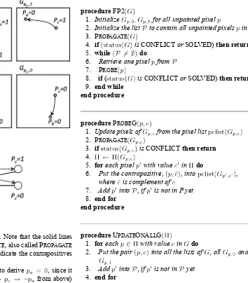
pixel relations are depicted in Fig. 4. Note that the solid lines indicate the derivations via PROPAGATE, also called PROPAGATE implications, and the dashed lines indicate the contrapositives in the rest of this paper.

From Fig. 3 (or Fig. 4), it is easy to derive , since it is true in both cases (due to from above) and (due to ). The result can also be derived in another way by showing a con_flict with the assumption , which leads to a contradiction . Unfor-tunately, the FP1 method cannot obtain this result . The FP1 method can only derive those solid lines, and, therefore, is unable to derive .

In order to solve this problem, we propose the second FP method, named FP2, to add the contrapositives into grids as fol-lows. In the new method, all grids, say , are associated with a list of pairs of pixels and their values, denoted by , used to record the derived values for given pixels, mainly for the contrapositive. For example, in Fig. 3, for , its con-trapositive is stored by putting the pair into . When probing a grid, update the cells of the grid from the list before using PROPAGATE. For example, if

contains , the routine PROBEprobing first sets the pixel to 0 from , and then performs PROPAGATE.

The next issue is when to probe a grid. For this issue, we maintain a list of pixels , denoted by , to indicate both grids to be probed. Whenever a new contrapositive is added into or , pixel is put into , unless is already in . The routine for FP2 is described as follows.

procedureFP2

1. Initialize for all unpainted pixel

2. Initialize the list to contain all unpainted pixels in

3. PROPAGATE

4. if isCONFLICTorSOLVED)then return

5. while do

6. Retrieve one pixel from

7. PROBE

8. if( isCONFLICTorSOLVED)then return 9. end while

end procedure

procedurePROBEG

1. Update pixels of from the pixel list

2. PROPAGATE

3. if isCONFLICTthen return 4.

5. foreach pixel with value in do

6. Put the contrapositive, ,into ,

where is complement of

7. Add into ,if is not in P yet

8. end for end procedure

procedureUPDATEONALLG

1. foreach with value in do

2. Put the pair into all the lists of ,all and, 3. Add into ,if is not in yet

4. end for end procedure

The FP2 method is changed as shown above. The routine PROBEis the same as the one in the FP1 method, except that the two routines PROBEG and UPDATEONALLG are modi_fied as shown above. Now, examine how FP2 can obtain in the example in Fig. 3. Here, we consider two situations. The_first sit-uation is to retrieve from earlier than . In this situation, probe is retrieved earlier than . When probing , store the contrapositive into . Next, when probing , set initially to be 0 in from the contrapositive , then perform PROPAGATE, which results in a con_flict due to both and . Thus, we establish that in line 7 of PROBE, and UPDATEONALLG is subsequently called in line 11 to set it to all grids including . The second situation is to retrieve _first from , then and . After probing and , two contrapositives and are stored in and , respectively. Next, when probing , we ob-tain from in . Since in both and , we establish that in line 9 of PROBE.

Fig. 5. (a) Puzzle given in [2]. (b) Initial where is in the upper left corner. (c) , where is in the middle of the rightmost column.

Fig. 6. An example modified from Fig. 5.

pixel in white in the middle row of the rightmost column, though six white pixels can be painted as shown in Fig. 5(a). For this puzzle, FP1 cannot paint it either. However, FP2 can paint in white in the following way. First, when probing pixel in the upper left corner, we can obtain , as shown in Fig. 5(b). This implies that . In FP2, we can obtain its contrapositive , and, similarly obtain . Then, when probing for the grid , as shown in Fig. 5(c), performing PROPAGATE in the leftmost column will paint (the middle of the leftmost column) in black, and then detect a con_flict in the third row. Hence, we establish that should be painted in white.

For this example, one might argue that the FP method would be suf_ficient if it simply returned a solution immediately, when probing on yields a valid solution, then continuing from . Assume that the aforementioned method is used instead. We can demonstrate that a solution is not guaranteed simply by probing. The example illustrated in Fig. 6 is similar to Fig. 5, except there are now extra rows in the bottom of the puzzle that cause no solutions to be found like that in Fig. 5. Again, in this example, FP2 can paint pixel , while FP1 and the method in [2] cannot.

The time complexity of FP2 remains only, as ex-plained in the following two aspects.

1) For each of the grids and all and , we still use incremental propagation to perform PROPAGATE, so the total time complexity for these is , as de-scribed in Section III-A.

2) The routine PROBE is also invoked times, since there are at most pairs of in total, and each pair of is put into the list at most

Fig. 7. Case where FP2 cannotfind .

times for the following reason. Each for the pair of grids is put into the list only when it is being initialized, or when at least one pixel is newly painted (in PROBEG or UPDATEONALLG) in both and , where there are at most pixels. In addition, at most contrapositives for each of the grids can be stored into pclist in line 6 in PROBEG, so the time for the loop between lines 5 and 8 is . Moreover, the time for UPDATEONALLG is , as described in Section III-A. Hence, the time for updating pixels in line 1 of PROBEG is as well.

From the above, FP2 can paint more pixels over FP1 without a higher tradeoff in terms of time complexity, while FP1 has the advantage of being easier to implement.

C. The Third FP Method

In this section, we further discuss some cases where the FP2 method cannot paint, and then propose a third method, named FP3. However, the tradeoff is an increase in the time complexity to , slightly higher than , where the value is nor-mally smaller than .

The FP2 method is able to deduce PROPAGATEimplications from contrapositives. For example, the contrapositive

in Fig. 7 helps deduce as follows. After the contra-positive is set from , the probing on results in in by deducing from to in PROPAGATE. Unfortunately, FP2 cannot perform deductions that are the other way around. That is, the contrapositive

does not help deduce , since it involves going from a PROPAGATEimplication to a contrapositive. Similarly, for the same reason, we cannot derive .

In fact, from PROPAGATE implications and their corre-sponding contrapositives in Fig. 7, condition obviously holds from the following two deductions:

or .

Unfortu-nately, using FP2, we can only derive two more, and , which do not contribute to the result of . In order to solve this problem, we use a technique such as graph traversal for solving 2-SAT [6] in the FP3 method as fol-lows. For a newly painted pixel in , say (implying ), all newly painted pixels in (with respect to ) are also updated and painted in . The update operation is done recursively for any newly painted pixels. For example, in Fig. 7, when updating in , also update and if both are already set in . The routine PROBEG in the method is modi_fied as follows.

Fig. 8. General deduction.

painted pixels from to , as described above, where are the painted pixels in , including those in list , but not in . Note that a con_flict occurs in when a pixel is set with different values. 2) In line 2, for each pixel that is newly painted with

in PROPAGATE, update all the newly painted pixels from to as above.

3) In line 4, add all the newly painted pixels in lines 1 and 2 into .

The above modi_fication ensures that all deductions via PROPAGATE implications and contrapositives can be found. Namely, in the case shown in Fig. 8, we can deduce the fol-lowing: 1) ; and 2) , for all .

Now, let us compare our method with the method proposed in [2] by Batenberg and Kosters without considering tomographic constraints.1 _{Using the above modifications for FP3, all the} pixels that are painted by their method as above can also be painted by FP3 for the following reason. Their method checks all relations between all pairs of pixels in the same lines (rows or columns) and then uses a 2-SAT method to derive more pixel relations, if any. In FP3, we probe a pixel with a color to derive all PROPAGATEimplications to other pixels, not limited to the same line, and then use the above update operation (a kind of 2-SAT operation) to derive more pixel relations, if any. Since probing a pixel with a color derives more pixel relations (not limited to the same lines), all the pixel relations obtained in their method [2] are also obtained in FP3.

The time complexity of this method becomes as ex-plained in the following. For the_first two modi_fication items in the routine PROBEG, as speci_fied above, the update operation for each newly painted pixel takes time to check whether grids and have more painted pixels to paint. Since the total number of newly painted pixels is , the total time for checking grids is .

D. Discussion

This section compares our methods (before backtracking) with those in [2]. From our analysis, the time complexity for each line solving, such as in [2] (using DP) is estimated to be , as mentioned above. In their 2-SAT method, they first calculated all the 2-SAT relations between any two pixels in the same line (rows or columns), and then used a 2-SAT algorithm to paint more pixels.

For the former, the method from [2] initially collects all the 2-SAT relations between any two pixels in the same line. It is easy to derive the number of pairs to be . Then, when-ever a pixel is painted, it is required to recalculate all 2-SAT relations on any pair of pixels in the column or row containing

1_{Although the method may possibly paint more pixels, our experiments show} little improvement, as discussed in Section V.

it. Thus, the number of recalculated 2-SAT relations due to this painted pixel is . Since at most pixels are painted, the total number of recalculated relations is . Thus, the total time for calculating 2-SAT relations is , which is higher than ours. Even if they use our line-solving method, the total time will still be , the same as those of FP1’s and FP2’s. For the latter, they used a 2-SAT algorithm to detect con_flicts and, therefore, paint more pixels. Starting from each among all pixels, the method is to explore a path to by traversing the graph with relations, as described above. Thus, it takes time to detect con_flicts for one round. Whenever one pixel is updated, the whole process needs to be performed for a new round. Thus, since there are at most pixels to be updated, the total time required is .

In regards to the number of pixels that are painted, our methods such as FP2 and FP3 are able to paint more pixels than the 2-SAT method. Examples are shown in Figs. 5 and 6. On the other hand, Section III-C also shows that all the pixels that the 2-SAT method can paint can also be painted by FP3. Our experiments in Section V also con_firm this.

IV. BACKTRACKING

In many puzzles, all pixels in the grids can be completely painted following an FP method: FP1, FP2, or FP3. However, if the grids are not completely painted, we still need to use the backtracking method to paint the whole grid. In our back-tracking method,_first, we use an FP method to paint as many pixels as possible. If a con_flict is not detected or a solution is not yet found in the grid, we use choose-pixel heuristics2_{in a} rou-tine named CHOOSEPIXELto choose the next pixel to extend. After choosing , we paint the value 0 to , then recursively call the backtracking method. The process is repeated similarly for painting 1 on . The routine BACKTRACKINGis written as follows.

procedureBACKTRACKING

1. INITIALIZEall and for all

2. FP3 ; // or FP1 , FP2

3. if isCONFLICT)then return 4. if isSOLVED)then

5. Continue to solve more or stop depending on the requirement.

The time complexity for backtracking is inherently exponen-tial in the worst case. Thus, careful consideration must be given when choosing the next pixel to extend in CHOOSEPIXEL, in order to achieve good performance. Fortunately, our FP

methods have an important feature: all the grids and are probed in advance; that is, all ’s are extended tentatively in advance. This feature offers more accurate information for choose-pixel heuristics. With this advantage, it is much easier to design choose-pixel heuristics when deciding which pixel to extend to. For example, we can choose pixel that maximizes , where value denotes the number of extra pixels painted in , not in . In general, the larger is, the better it is to extend on . This is because extending on with generally results in more pixels painted. We tried many choose-pixel heuristics in our experiments in Section V.

V. EXPERIMENTS

We performed experiments to analyze our methods for nono-gram solvers, the results of which are described in this sec-tion. Most of our experiments were run using an Intel® Core™ i5-2400 CPU 3.10 GHz. In our experiments, two main sets of test puzzles were used for performance analysis. The_first set contained 1000 25 25 puzzles generated at the TAAI 2011 Nonogram Solver Tournament [10], [16]. In this tournament, a nonogram random generator [23] was used to produce these puzzles at random, where the density of black cells in these 1000 puzzles ranged from 50% to 35%, in linearly decreasing order. It is worth noting that these puzzles do not guarantee unique solutions. According to [2], the most dif_ficult puzzles contain about 20%–35% black cells; the higher the density of black cells (more than 35%), the easier the puzzles are. This implies that the generated puzzles (from 50% to 35%) were ordered roughly from easy to hard.

The second set contained 100 puzzles produced by Wu [23] in another nonogram tournament at TAAI 2011, where each partic-ipant generated 100 puzzles for opponents to solve. These puz-zles were required to have unique solutions and were usually much harder. For simplicity of analysis, nonogram programs were required to_find second solutions for all the puzzles. Since these puzzles all had unique solutions, the programs were forced to search completely.

In our experiments, the various choose-pixel heuristics that were tried are listed as follows.

1) Sum: Choose

2) Min: Choose

where .

3) Max: Choose

where .

4) Mul: Choose

5) Sqrt: Choose

6) Min-logm: Choose

where .

7) Min-logd: Choose

In our experiments, we also supported caching for all lines, as suggested in [20], since the solving of identical lines is highly likely. For example, a row to be solved may be the same as one already solved earlier. Since caching is not the core of this paper, we simply use a suf_ficiently large cache.

The experimental results are shown in Section V-A. Section V-B compares our nonogram solver with other solvers.

A. Performances of Test Cases

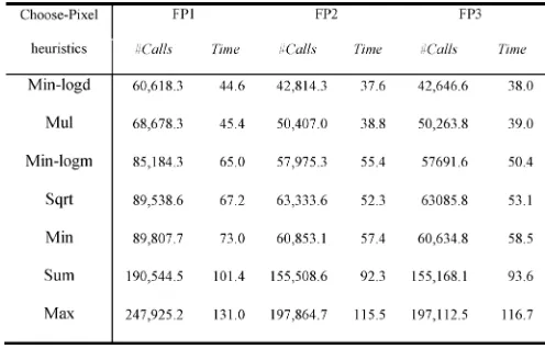
In this section, the two sets of puzzles were run with the seven choose-pixel heuristics and with the three FP methods, FP1, FP2 and FP3, respectively. The results are shown in Tables I and II, and the average times in Tables I and II are depicted in Fig. 9. The columns for “#Calls” indicate the average number of back-tracking calls (calls to BACKTRACKING), and those for “Time” indicate the average time in seconds taken for each puzzle. In Tables I and II, the heuristics are sorted according to the corre-sponding times of FP3.

From Tables I and II, we discuss the results in the following three aspects. First, the number of calls for FP1 is generally higher than that for FP2 by a factor of 30%, while that for FP2 is very close to, speci_fically only 1% higher than, that for FP3. The results show that the improvement from FP1 to both FP2 and FP3 is signi_ficant and that from FP2 to FP3 is less signi_fi -cant. This implies that a signi_ficant improvement is achieved by adding contrapositives in FP2, as described in Section III-B. In contrast, propagating all the PROPAGATEimplications and con-trapositives in FP3 does not yield much improvement.

Second, in terms of computation time, both FP2 and FP3 run, in general, faster than FP1 by a factor of 19%. In fact, the FP2 method incurs some overhead over FP1 in maintaining a list of pixel values. The average time taken for each call in FP1 is about 0.55 ms, while those in both FP2 and FP3 are about 0.60 ms. The overhead for FP2 and FP3 is incurred by the maintenance of the data structure for . FP3 runs only 1% faster than FP2. Although the overhead incurred by FP3 (over FP2) is high in theory, as shown in Section III-C, in practice the overhead is actually low if bitwise operations are used. The results show that the additional overhead for FP3 is less signi_ficant.

Fig. 9. The average times for all heuristics using FP1, FP2, or FP3 for (a) the

first set and (b) the second set.

TABLE I

PERFORMANCERESULTS FOR THEFIRSTSET OFTESTCASES

Next, we wanted to investigate the performance of FP methods from the perspective of the average numbers of painted pixels before backtracking. Table III shows the average numbers of painted pixels, after the initial PROPAGATEon the grid and the_first call to FP1, FP2, and FP3, respectively. The experimental results for the _first set show that the initial PROPAGATEcan solve only 32 pixels on average, but the three

TABLE II

PERFORMANCERESULTS FOR THESECONDSET OFTESTCASES

TABLE III

THEAVERAGENUMBERS OFPAINTEDPIXELSAFTERINITIALPROPAGATE,

THE2-SAT METHOD IN[2], FP1, FP2,ANDFP3

methods FP1, FP2, and FP3 improve by painting 201–211 pixels, about 170 more pixels. The results also show that both FP2 and FP3 are clearly better than FP1 by solving 9.4 and 10.1 more pixels on average, respectively. However, the improve-ment from FP2 to FP3 is very small, with only 0.7 more pixels on average. For the second set, the experimental results show a similar relation. However, since the set of puzzles is more dif_ficult, the numbers of painted pixels are generally smaller than those in the_first set.

Next, we wanted to compare our method with the method pro-posed in [2] without DT (as mentioned in Section III-C). In the column “2-SAT” of Table III, the values indicate the average numbers of painted pixels after _finishing the 2-SAT method. From the table, FP3 can solve 116.4 more pixels on average for the_first set and 23.7 more pixels for the second set. This shows that our FP methods can paint many more pixels than theirs, while our methods also perform more ef_ficiently (as described in Section III-D). In addition to 2-SAT, Batenburg [1] and Baten-burg and Kosters [2] also proposed a DT method to help paint more pixels. However, our experiments also show that a 2-SAT method together with DT solves almost the same number of pixels as that for the 2-SAT method alone, but it takes much more time. More speci_fically, for all the puzzles in the above two sets (1100 puzzles), the 2-SAT method with DT can paint in total only_five more pixels than the 2-SAT method. This shows that DT is not critical when attempting to paint more pixels.

B. Comparison to Other Solvers

TABLE IV 5000 PUZZLESGIVEN IN[21]

1000 puzzles from the TAAI 2011 Nonogram Solver Tourna-ment, as mentioned in Section V-A. In this tournaTourna-ment, our pro-gram named LALAFROGKK solved all 1000 puzzles in 645 s [10] on a machine equipped with Intel® Core™ i7-970 CPU 3.60 GHz, and outperformed the other two teams, YAYAGRAM and NAUGHTY. YAYAGRAMsolved 766 puzzles in 120 min (the time limitation of this tournament), while NAUGHTYsolved 509 puzzles.

Second, consider the set of 5000 puzzles generated by a nonogram random generator in [21] where the density of black cells is about 50%. The site also collected many public nono-gram solvers, including NAUGHTY, but not yet LALAFROGKK. NAUGHTYwas ranked the fastest among all the programs on this site, and PBNSOLVEwas ranked the second fastest. Table IV shows the computation times of the two programs as well as ours, after we reran all 5000 puzzles for all three solvers on an Intel® Core™ i5-2400 CPU 3.10 GHz. The result shows that the average computation time for LALAFROGKK is the fastest one, and that the number of puzzles that required over 1 min to solve is only one for LALAFROGKK, but_five for NAUGHTY and 21 for PBNSOLVE.

VI. CONCLUSION

This paper proposes some methods to design an ef_ficient nonogram solver. The contributions are listed as follows.

1) We propose a fast DP method for line solving, whose time complexity in the worst case is only, where the grid size is , and is the average number of integers in one constraint, always smaller than . In contrast, the DP method in [2] is .

2) We propose three FP methods, named FP1, FP2, and FP3, respectively, to solve more pixels before backtracking. This contribution has signi_ficant value in the following two senses. First, both FP2 and FP3 can solve more pixels than the method in [2] (before backtracking), while the time complexities for FP2 and FP3 are faster than theirs by a factor of .

Second, these FP methods can provide backtracking with useful guidance when choosing the next pixel to guess. Our experiments also showed that FP3 performed the fastest, improving performance over FP1 signi_ficantly, but improving performance over FP2 only slightly.

3) We incorporate the proposed methods into a fast nono-gram solver, named LALAFROGKK, which won a nono-gram tournament at TAAI 2011. In addition, in the 5000 test cases given in [21], our program clearly outperformed other programs collected in [21].

The FP method proposed in this paper is actually a generic method for many puzzle problems. In practice, we are applying this method to some other puzzle problems such asNurikabe

[22],Slitherlink[12], andSudoku[11]. We believe this method is an important generic method for solving puzzles like dancing links [9].

APPENDIX

In this Appendix, we design a line-solving algorithm whose time complexity is . We follow the de_finitions and no-tation in Section II-B2. The algorithm maintains three arrays: , and . Each , initialized to be false, indicates whether there exists some_fix with the th pixel 0. Similarly, each indicates for the th pixel 1. Each is the lowest index such that are all 1’s.

The algorithm starts calculating from , and uses memorization to prevent repeatedly calculating recurrences for both and , as described in [7].

is calculated only when is true. Similarly,

is calculated only when is true, and is calculated only when is true.

Assume that is true. Then, set must be nonempty. This implies that there exists some with the th pixel 0, and this also implies that there exists some with the th pixel 0. Thus, in , also set to true.

Similarly, assume that is true. Then, set must be nonempty. This implies that there exists some such

that . Since , we

have and . A straightforward

method for is to set to true, and set all to true. However, the computation time increases the order, using this method. So, we set

to true, and to . If

is lower than the original becomes

to indicate implicitly that all are set to true. On the other hand, if the original is lower than , all of these are implicitly set to true already, so no more operations are needed.

When is completed,_first, we scan all from back to and set the corresponding according to . It is not hard to perform the above operation in linear time. Then, determine the_final by merging all and

, in the following way. For all , if is true and is false, set ; if is false and is true, set ; and if both and are true, set . Note that it is impossible to have both and to be false, since set

is nonempty if is true.

The time complexity of the above algorithm is only for the following reason. The time for merging all and

is . Thus, the total time for calculating all

and is .

ACKNOWLEDGMENT

The authors would like to thank the anonymous referees and T.-Han Wei for their valuable comments.

REFERENCES

[1] K. J. Batenburg, “A networkflow algorithm for reconstructing binary images from discrete X-rays,”J. Math. Imag. Vis., vol. 27, no. 2, pp. 175–191, 2007.

[2] K. J. Batenburg and W. A. Kosters, “Solving nonograms by com-bining relaxations,”Pattern Recognit., vol. 42, no. 8, pp. 1672–1683, 2009.

[3] K. J. Batenburg, S. Henstra, W. A. Kosters, and W. J. Palenstijn, “Con-structing simple nonograms of varying difficulty,”Pure Math. Appl., vol. 20, pp. 1–15, 2009.

[4] F. Bacchus and P. van Run, “Dynamic variable ordering in CSPs,” in Principles and Practice of Constraints Programming (CP-95), ser. Lecture Notes in Computer Science. Berlin, Germany: Springer-Verlag, 1995, vol. 976, pp. 258–277.

[5] R. A. Bosch, “Painting by numbers,”Optima, vol. 65, pp. 16–17, 2001. [6] D. Cohen, P. Jeavons, and M. Gyssens, “A unified theory of structural tractability for constraint satisfaction problems,”J. Comput. Syst. Sci., vol. 74, no. 5, pp. 721–743, 2008.

[7] T. H. Cormen, C. E. Leiserson, R. L. Rivest, and C. Stein, Introduction to Algorithms, 3rd ed. Cambridge, MA, USA: MIT Press, 2009. [8] F. Faase, “Nonogram to exact cover,” [Online]. Available: http://www.

iwriteiam.nl/D0906.html#28

[9] D. E. Knuth, “Dancing links,” inMillenial Perspectives in Computer Science. Basingstoke, U.K.: Palgrave, 2000, pp. 187–214. [10] H.-H. Lin, D.-J. Sun, I.-C. Wu, and S.-J. Yen, “The 2011 TAAI

com-puter-game tournaments,”Int. Comput. Games Assoc. J., vol. 34, no. 1, pp. 51–54, 2011.

[11] H.-H. Lin and I.-C. Wu, “An efficient approach to solving the minimum Sudoku problem,”Int. Comput. Games Assoc. J., vol. 34, no. 4, pp. 191–208, Dec. 2011.

[12] T.-Y. Liu, I.-C. Wu, and D.-J. Sun, “Solving the slitherlink problem,” inProc. Conf. Technol. Appl. Artif. Intell., 2012, pp. 284–289. [13] M. Olšák and P. Olšák, “Griddlers solver,” [Online]. Available: http://

www.olsak.net/grid.html#English

[14] The Puzzle Museum, “Origins of cross reference grid & picture grid puzzles,” 2012 [Online]. Available: puzzlemuseum.com/griddler/grid-hist.htm

[15] S. Simpson, “Nonogram solver,” [Online]. Available: www.comp. lancs.ac.uk/~ss/nonogram/

[16] D.-J. Sun, K.-C. Wu, I.-C. Wu, S.-J. Yen, and K.-Y. Kao, “Nonogram tournaments in TAAI 2011,”Int. Comput. Games Assoc. J., vol. 35, no. 2, Jun. 2012.

[17] N. Ueda and T. Nagao, “NP-completeness results for nonogram via parsimonious reductions,” Dept. Comput. Sci., Tokyo Inst. Technol., Tokyo, Japan, Tech. Rep. TR96-0008, 1996.

[18] W. A. Wiggers, “A comparison of a genetic algorithm and a depthfirst search algorithm applied to Japanese nonograms,” inProc. Twente Stu-dent Conf. IT, Jun. 2004, pp. 1–6.

[19] Wikipedia, “Nonogram,” [Online]. Available: en.wikipedia.org/wiki/ Nonogram

[20] J. Wolter, “Effect of line solution caching on Pbnsolve run-times,” [On-line]. Available: http://webpbn.com/survey/caching.html

[21] J. Wolter, “The ‘Pbnsolve’ paint-by-number puzzle solver,” [Online]. Available: http://webpbn.com/pbnsolve.html

[22] I.-C. Wu, D.-J. Sun, and S.-J. Yen, “HAPPYNURI wins Nurikabe tour-nament,”Int. Comput. Games Assoc. J., vol. 33, no. 4, p. 236, Dec. 2010.

[23] K.-C. Wu, “TAAI2011 Nonogram Tournament result,” 2012 [Online]. Available: http://kcwu.csie.org/~kcwu/nonogram/taai11/

[24] C.-H. Yu, H.-L. Lee, and L.-H. Chen, “An efficient algorithm for solving nonograms,”Appl. Intell., vol. 35, no. 1, pp. 18–31, 2009.

I.-Chen Wu(M’10) received the B.S. degree in elec-tronic engineering and the M.S. degree in computer science from the National Taiwan University (NTU), Taipei, Taiwan, in 1982 and 1984, respectively, and the Ph.D. degree in computer science from Carnegie Mellon University, Pittsburgh, PA, USA, in 1993.

Currently, he is with the Department of Computer Science, National Chiao-Tung University, Hsinchu, Taiwan, and also serves as the Director of the Institute of Multimedia Engineering. His research interests in-clude artificial intelligence, Internet gaming, volun-teer computing, and cloud computing.

Dr. Wu introduced the new game,Connect6, a kind of six-in-a-row game, in 2005. Since then,Connect6has become a tournament item in the Computer Olympiad. He led a team developing various game-playing programs, winning over 20 gold medals in international tournaments, including the Computer Olympiad. He wrote over 80 papers, and served as a chair and a committee member in over 30 academic conferences and organizations, including the Games Technical Committee of the IEEE Computational Intelligence Society.

Der-Johng Sunreceived the M.S. degree in botany from the National Taiwan University (NTU), Taipei, Taiwan, in 1996. He is currently working toward the Ph.D. degree in computer science at the National Chiao-Tung University, Hsinchu, Taiwan.

His research interests include information extrac-tion, artificial intelligence, and cloud computing.

Lung-Pin Chenreceived the B.S. degree from Soo-chow University, Suzhou, Jiangsu, China, in 1991, the M.S. degree from the National Chung-Cheng University, Minxueng, Chiayi, Taiwan, in 1993, and the Ph.D. degree from the National Chiao-Tung Uni-versity, Hsinchu, Taiwan, in 1999, all in computer science.

He is an Associate Professor at the Department of Computer Science and Information Engineering, Tung-Hai University, Taichung, Taiwan. His re-search interests include distributed algorithm, service computing, and pervasive computing.

Kan-Yueh Chenreceived the M.S. degree in com-puter science from the National Chiao-Tung Univer-sity, Hsinchu, Taiwan, in 2012.

His research interests include artificial intelligence and cloud computing.

Ching-Hua Kuoreceived the M.S. degree in com-puter science from the National Chiao-Tung Univer-sity, Hsinchu, Taiwan, in 2012.

Hao-Hua Kangreceived the M.S. degree in com-puter science from the National Chiao-Tung Univer-sity, Hsinchu, Taiwan, in 2012.

His research interests include artificial intelligence and cloud computing.

Hung-Hsuan Lin received the B.S. degree in computer science from the Department of Computer Science, National Chiao-Tung University, Hsinchu, Taiwan, in 2007, where he is currently working toward the Ph.D. degree in computer science.