Issues
ISSN: 2146-4138
available at http: www.econjournals.com
International Journal of Economics and Financial Issues, 2017, 7(1), 566-574.
The Dynamic Impact of Trade Openness on Poverty: An
Empirical Study of Indonesia’s Economy
Lestari Agusalim*
Department of Economic Development, Faculty of Economics Business and Humanities, Trilogi University, Jakarta, Indonesia. *Email: [email protected]
ABSTRACT
This research aims to analyze the dynamic impact of international trade openness on poverty in Indonesia. Previous research shows different effects in every country. The data used are export import value, gross domestic product, income per capita, open unemployment rate (OUR), and poverty rate
(POVR) during 1978-2015. Vector error correction model analysis shows that in short run, trade openness does not have any signiicant impact on poverty. However, in long run, it has signiicant impact in reducing poverty. Impulse respond function analysis concludes that POVR gave a positive response in the irst 2 years, but negative in the third to every trade openness variable shock. Poverty rate shows the biggest negative response in the ifth year. According to forecast error variance decomposition analysis, trade openness does not give big contribution in affecting POVR during the irst 3 years, but starts to show effect in the following seven, with the biggest in the ninth year.
Keywords: Trade Openness, Poverty, Vector Error Correction Model
JEL Classiications: C10, F14, I32
1. INTRODUCTION
Economic Globalization is an integrating process of national
economy into a global economy system (Fakih, 2002). It is marked
by the raising of a country’s economic openness to international trade. The economic globalization will create an interplay
economic relation, also goods and services low will shape the
trading between countries. The control from government will fade because the globalization process is moved by the global market power, not by the policy or regulation from government individually. The trade openness will affect a country’s economic growth because all nations will compete in international market
(Todaro and Smith, 2006).
According to Huczynski and Buchanan (2007), economic
globalization created a rapid change situation. From cyber revolution, trade liberalization, goods and services homogenization in the whole world, to export which oriented to international trade growth were the components of globalization phenomenon. However, it often created strong impacts to income pattern in a country. The international trade is believed to contrive the
beneiciaries and the injured party.
Globalization has both positive and negative impacts. The positive impacts of it are the increasing of national income due to the comparative advantage, the entry way to global capital, technology diffusion, human rights transmittal and escalation of job opportunity so that able to up lift the welfare in a nation. Based on those ideas, international trade organization and economists say that globalization will push the economic growth and reduce the poverty. Meanwhile, the negative impacts of globalization are the weakening the less skilled and less capital countries, weak management in international trade of a underdevelopment country, workers exploitation in developing country, unstable global capital market risk, national culture stability weakening, national economy autonomy which is destructed by stock market disclosure, and the underdevelopment country should accept the regulations made by the developed country (Mutascu and
Fleischer, 2011).
Economic globalization is undeniable by every country in the
world, because of the free trade, information low, the goods
and services between countries increasing the economic growth.
free trade area (AFTA), Asia-Paciic Economic Cooperation in
1994, World Trade and Organization in 1995. There were also
additional collaborations from AFTA such as ASEAN-China free trade, ASEAN-Korea free trade, ASEAN-India free trade, ASEAN-Australia-New Zealand AFTA and ASEAN-Japan comprehensive economic partnership. By the end of 2015, Indonesia entered the ASEAN Economic Community era
where free trade was created in capital, goods and services, also
workforce as the follow-up of AFTA.
The number of ratiications of international economic cooperation
by Indonesia had caused the discourse among the economists specially regarding to the impact of economic openness to poverty rate (POVR) in the country. Figure 1, shows the trends
of export, import, and POVR in Indonesia since 1978-2015.
For 38 years, Indonesia’s export import experienced a rapid increasing. Indonesia trade balance was always in positive mark
except in 2012-2014 which experienced the deicit trade balance. One of the factors which caused the deicit pressure on it was the
increasing demand for imported oil and gas commodities, and the declining performance of non-oil and gas export (Ginting,
2014). Furthermore, it was also driven by the increasing demand
for motorized vehicle and smart phone. Meanwhile, the POVR
in Indonesia went through luctuation, in new order era there was a signiicant decreasing on POVR. During the transition to
reformation era there was an increasing POVR caused by monetary
crisis and politic. However, after 2001 the POVR was decreasing
in a slow pace.
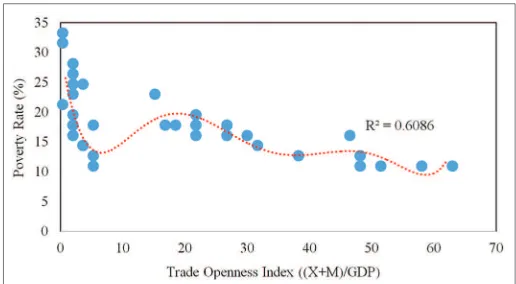
Furthermore, Figure 2 shows the early correlation detection between economic globalization as proxied by trade openness index (TOI) (export value ratio and import to gross domestic product [GDP]) and POVR in Indonesia. The igure shows the trend that when Indonesia continues to open up to international trade, poverty tends to decrease. However, there is no chance to conclude based on those correlations. It could be just a pseudo-relation so it requires a deeper and accountable study.
Based on the background described, it is interesting to observe more about the trade openness and its dynamic impact on poverty in Indonesia. It will provide substantial information for government to examine the Indonesia’s economic direction. Besides the introduction, the rest of the paper proceeds as follows. Section 2 provides a review of the related literature. Section 3 contains the empirical methodology adopted for this study. Section 4 empirical estimation and results. Section 5 presents some concluding remarks.
2. LITERATURE REVIEW
There is a polemic on the advantage and disadvantage of trade openness. Based on some researches which were conducted in many countries, found that there were 3 patterns of connection between trade openness and poverty in a country, such as; (1) trade openness cause the poverty decreasing, (2) trade openness cause the poverty increasing, (3) there is a complicated connection between trade openness and poverty.
The impact of trade openness in decreasing the poverty was
proved by the researches of Ozcan and Kar (2016), Okungbowa and Eburajolo (2014), Oyewale and Amusat (2013), and Fischer (2003) who found that trade openness was able to push the
economic growth and decrease the poverty in the world. Most of the economists and economic organization said the same as well. The ones who pro to the international trade claimed that
the globalization wave since 1980s had promoted the economic equality and reduced the POVR (Dollar and Kraay, 2002).
Ozcan and Kar (2016) conducted a research on the impact of trade
liberalization on poverty in Turkey. Turkey started to implement
the export oriented growth in the early 1980s and had become the
integral part of world economy. Trade liberalization was hoped to lift up the economic growth, income per capita, and reduce the poverty. By using the vector error correction model (VECM) model, found that trade liberalization reduced the poverty in Turkey.
Okungbowa and Eburajolo (2014) also found the same result
when conducting the research in Nigeria. Economic globalization
caused the reduction POVR. So did Oyewale and Amusat (2013)
who marked globalization through the wide spreading of economy integration to lift up the living standard in the whole world,
however, most of the developing country in Africa, Asia, and Latin America had become the victim of globalization process mostly
Figure 1: Export, import, and poverty rate
Source: BPS-Statistics Indonesia and Ministry of Trade, 2016
(data processed)
Figure 2: Correlation between trade openness index and poverty rate
Source: BPS-Statistics Indonesia and Ministry of Trade, 2016
because of the poverty and inequality income which increased in the last two decades.
However, there were doubts from the contras group who claimed that globalization made country getting poor. Result of the
researches by Chen and Ravallion (2007), Ravallion (2006), Abbott (2003), and Twyford (2003) showed that poverty was still
high as the growth of economic globalization. Chen and Ravallion
(2007) made arguments which doubting that globalization was able to decrease the poverty in underdeveloped country. As the
prove, poverty was still high in many underdeveloped countries after the globalization current spread even though the number of people below the absolute poverty line kept decreasing. People
who lived under $1 per day in the world decreased from about 30% in 1981 to 18% in 2004 in Asia. Meanwhile, the absolute poverty decreased from 11% to 9% in Latin America and Caribbean, 42-41% in Sub-Sahara Africa, and 0.7-0.9% in Eastern Europe and Central Asia.
In Ravallion research (2006) which used the POVR data and TOI
from many countries in a long run, showed there was not any
signiicant correlation between POVR and TOI. The result of the
empiric approach doubted that the growing of the international trade openness would decrease the poverty precisely. The conclusion of that research showed that it was not easy to prove that there was a strong correlation between trade openness in reducing the poverty in underdeveloped countries. It was because there was political policy in underdeveloped country which weakened the connection between trade liberalization and poverty there. Meanwhile, in developed country the poverty was decreasing due to the trade liberalization.
Abbott (2003) found the same on his research. Result showed that
the world trade system was bias for the poor. They often subjected to greater trade tariffs than the wealthy people. The political policy of the developed country caused the underdeveloped country got
hard to get out of the poverty. Twyford (2003) explained that
the POVR was not only affected by trade liberalization, but also depended on many factors, such as the initial distribution of income and asset, what is produced, bought, and consumed by poor, and
how the competitiveness of national producer in world trade. As
an example, in Nepal, there was a rapid trade openness but was
not able to decrease the poverty signiicantly.
Another research conducted by Chaudhry and Imran (2013), Nissanke and Thorbecke (2010), Harrison (2007), Harrison et al., (2004) and Lopez (2004) found that there was a complex
and blur relation between economic globalization and poverty.
Chaudhry and Imran (2013) conducted a research in Pakistan
using time series regression analysis found an empirical evidence that trade liberalization decreased the poverty but did not have
signiicant impact statistically to poverty in short run. In long
run, trade liberalization had several strong effects on poverty.
Nissanke and Thorbecke (2010) said that globalization impact on
poverty was really complex relating to globalization interaction,
economic growth, and inequality. Lopez (2004) said that economic
integration could give a complicated effect on the connection among economic growth, poverty, and inequality.
Another study concluded that globalization could solve the poverty
matter if the complementary policy included the human resources development and infrastructure, and ongoing macro-economy
stability (Harrison, 2007). Globalization made worse the income
inequality, while the potential growth is limited so that increasing
the poverty in long run (Harrison et al., 2004). Globalization
could also discipline the government and limit the corruption, and check the negative side effect of growth inequality. It showed us that we should consider the complex interaction and relation among economy globalization, inequality, and economic growth, in checking the effect of globalization on poverty.
3. METHODOLOGY
The data used was the secondary data of the time series from 1978
to 2015. It was taken from BPS and Indonesia Ministry of Trade.
The literature review was taken from national and international
journal, books, and other scientiic literature. The data used was
the proxied economic growth to the GDP at constant price at the
base year 2010. The data TOI was proxied by the number of export
and import as the ratio of GDP. The POVR was proxied on the
data of poor ratio to the number of population. Another additional
data used was the income per capita proxied by the ratio of GDP
to the number of population. Last, the open unemployment rate
(OUR) data proxied from the number of unemployment to the number of labor force.
3.1. VECM Method
The method used to analyze on this research is VECM method.
VECM is the restricted VAR model which is used for
non-stationary variable but has co-integrated potential. It is suggested to input the co-integrated equation into the model which is being used after the test on the model. Most of the time series data have
stationary on irst difference or I (1). Later on, VECM utilizes the co-integrated restricting information into its speciication. Therefore, VECM often said as the VAR designed for the
non-stationary which has co-integrated connection. Furthermore, there is speed of adjustment in VECM from short run to long run. The
analysis tool which provided by VAR/VECM conducted through
four types of usage, such as forecasting, Impulse Respond Function (IRF), forecast error variance decomposition (FEVD), and granger
causality test (Firdaus, 2011). This research used support of Microsoft Excel 2016 software and Eviews 8.
The general VECM model speciication is:
k-1
Where yt is vector which contains the variable analyzed in the
research, μ0x is intercept vector, μ1x is coeficient regression vector, t is time trend, Πx is αxβ’, where β’ consist the long run
co-integrated equation, yt−1 is variable in level, Γix is coeficient
matrix, k−1 is VECM ordo from VAR, and et is et error term.
A pre-test estimating was conducted before doing the VAR
to ensure the data used so that estimation could produce a reliable data. The model regression which use non-stationary data would cause spurious regression (high R2, t-statistic, and signiicant F-statistic but dw relatively small <0.5). There are three criteria
of data to fulill the stationarity test, which are median (average)
and constant variant over time, and variance (covariance) between two rows of data but depends on the lag between those periods. The regression looks good but actually not, and could cause auto correlation. There are methods to conduct stationarity test, such
as Dicky-Fuller (DF test), Augmented DF (ADF test), and many others. On stationary test by ADF test, it uses real ive percent level. ADF can be tested with equation as below (Juanda and Junaidi, 2012):
∆Yt=β1+β1t+δYt−1+α1∆Yt−1+α2∆Yt−2+...+αi∆Yt−i+et (2)
Hypothesis used is H0: (which means Yt non-stationary); H1:
(which means Yt stationary). The t-statistic score which is got later
should be compared with t-McKinnon critical values. If t-statistic
less than t-table, H0 is accepted or there is not enough evidence to refuse hypothesis that in equation contains root unit, means the data is not stationary, and so did the other way.
Furthermore, another optimal lag test is conducted to create a good
VAR model with determining the number of optimal lag which used in the model. Lag in the VAR system is an essential matter
because the endogenous variable from endogenous variable in the equation system will be used as exogenous variable (Enders,
2004). The optimal lag length test can use several information such as Akaike information criterion (AIC), Schwartz Information
Criterion (SC), and Hannan-Quinn Criterion (HQ), the chosen lag is the smallest value in the model, too many lag will decrease the degree of freedom. Nevertheless, smaller lag is suggested to use
in order to reduce the error speciication.
The model stability test is conducted after conducting the optimal lag test in hope the whole roots have smaller modulus (absolute score) from one and placed on the unit circle. Nonetheless, the
VAR model is stabile so when doing an IRF and FEDV analysis
will have a valid estimation.
Last, co-integrated test is conducted to ind whether the
non-stationary variables co-integrated or not. The integration concept was stated by Engle and Granger (1987) as the linear combination from two or more non stationary variables would produce stationer variable. It is known as co-integrated equation and can be interpreted as long run equilibrium connection among variables. The co-integrated test using Johansen approach compares the
trace statistic and used critical value (which is 5%). If trace
statistic > critical value, the variable is co-integrated. VECM can be preceded after the number of co-integrated equation is known.
Estimating innovation accounting IRF and FEVD are conducted after doing the pre-test estimating. IRF is a model which is used to determine the response of an endogenous variable to a certain
luctuation variable (Amisano and Carlo, 1997). IRF is also used to see the effect of a certain luctuation variable to another variable
and how long (period) the effect lasts. It is due to the shock
variable for example that variable not only affect to itself, but also transmitted to every other endogen variable through dynamic structure or lag structure in a model.
FEVD is a model to see the strength and weakness of each variable affects other variable in a long run. The FEVD analysis is used to calculate and analyze how big the impact of random shock from
certain variable to endogen variable (Amisano and Carlo, 1997).
FEVD produces information about the importance of each random innovation structural disturbance or how strong a composition from certain variable role to other variable in VECM model.
3.2. Research Model
On this research, both of the short run and long run relevancy between trade openness and poverty in Indonesia appears, so the equation model is:
Where POV represent POVR, TOI is TOI, LNGDP is gross domestic product (in natural logarithm), LNGDP_C is gross domestic product
per capta (in natural logarithm), and UNEMP is OUR.
All the data used in VECM are in natural logarithm (LN) except the
percentage data. It is also to simplify when doing IRF and FEVD analyzing, the shock effect in standard deviation can be converted
in percentage. All variables in VECM method are the endogenous
variables, so in this research there is an interdependence connection among all variables.
4. EMPIRICAL ESTIMATION AND RESULTS
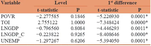
An examination to data stationarity test, optimal lag determination, and co-integrated test are conducted before examining the VAR estimation. The data stationarity test uses ive percent level. If t-ADF smaller than MacKinnon critical value, it can be concluded
that the data used is stationary (does not have unit root). The unit
root test is conducted on the level to irst difference. The result of
stationarity test can be seen on Table 1.
The amount of lag in VAR system is an essential matter. The lag
determination is not only useful to show how long the reaction of a variable to others, but also to remove the auto correlation problem
in a VAR system. The optimal lag determination generally based on the AIC, inal prediction error (FPE), HQ Information Criterion,
and SC. Based on Table 2, the smallest value for LR, FPE, AIC, and HQ criteria is on lag 4, while the smallest value for SC is on lag 1. The lag 4 will be used on this research because there are 4 recommended criteria.
The VAR stability test is conducted to gain the valid result on IRF and FEVD. The VAR model is stabile if the root has modulus
score (absolute score) <1. It shows the score is <1, which is
this research is stable. Nevertheless, the IRF and FEVD test can produce the valid output.
The co-integrated test is conducted to determine whether the
stationer variables on the irst difference are co-integrated. It
used the Johansen Co-integration Test by comparing the trace
statistic with the critical value 5%. If the trace statistic value is
higher than the critical value then there is a co-integrated in the equation system.
Based on Table 3 the model used on this research has four co-integrated equation. It shows that among those tested variables there is a stationary linear relation (co-integrated) in long run. Furthermore, this research can use the VECM model because
all the stationer data are on the irst difference and there is a
co-integrated among variables.
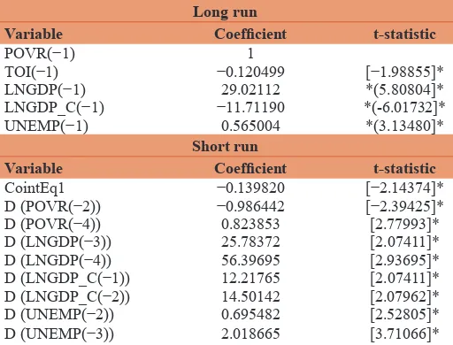
4.1. VECM Model
Besimi et al., (2006) said that the VECM model produces two main
estimations, which are measuring the short run connection among variables, and measuring the error-correction or the movement of variables speed to the long run equilibrium. Nonetheless, the VECM estimation is conducted to igure out the short run equilibrium relation and long run among variables. From the VECM estimation, it can obtain the short run relation and long run
relation among POVR, TOI, economic growth (LNGDP), income per capita (LNGDP_C), and OUR.
Table 4 shows the short run and long run variable connection.
Based on it, there are four signiicant inluential variables to the
POVR. Those are the POVR variables on the second and fourth
lag. On the second lag there is a negative signiicant inluential on
POVR, which means a one percent increasing on the two previous
years would decrease 0.98% POVR itself on this period. While on the fourth lag there is a positive signiicant inluential to POVR,
which means a one percent raise on the previous 4 years would
increase 0.82% POVR itself on this period.
The second variable is economic growth on the third and fourth
lag which has a positive signiicant inluence on POVR. It means
a one percent raise on the previous 3 years would increase 25.78% POVR on the ongoing year. As well as the fourth lag, if there is a 1% raise on the previous 4 year, would increase 56.39% POVR
on the ongoing year.
The third variable is the income per capita on the irst and second lag which has positive signiicant inluence on POVR. It means
a one percent raise on income per capita on the previous year
would increase 12.21% POVR on the ongoing year. As well as
the second lag, if there is a one percent raise on the income per
capita on the two previous years would increase 14.50% POVR
on the ongoing year.
The fourth variable is the OUR on the second and third lag which
has positive inluence on POVR. It means a one percent raise on OUR on the two previous years would increase 0.69% POVR on the ongoing year. As well as the third lag, if there is a 1% raise on OUR on the three previous years would increase 2.01% POVR
on the ongoing year.
Other useful information from the short run VECM estimation
result is the international trade openness does not have signiicant inluence to POVR in short run. It shows that trade openness cannot just decrease the poverty in Indonesia. According to McCulloch et al. (2001) trade which led to the trade liberalization is not
directly involved in solving the poverty. It just plays the minor role despite the trade openness is bigger. Therefore, the government’s policy is led to the trade liberalization, and should be followed by other anti-poverty policy so that trading can give maximum
beneit in reducing the poverty.
From Table 4, it can be seen that there is an adjusting mechanism from short run to long run which shown by significant
co-integration coeficient and has negative point. Coeficient on that co-integration means the error is corrected by 0.13% to get
the long run equilibrium. The long run VECM estimation result
shows that the variable which signiicantly inluence the POVR (POVR) in Indonesia is the TOI, economic growth (LNGDP), income per capita (LNGDP_C), and OUR (UNEMP).
The long run connection above can be written in the linear equation below:
POVR = −0.12* TOI + 29.02* LNGDP – 11.71*
LNGDP_C + 0.56* UNEMP (4)
On VECM test, the TOI variable has negative effect signiicantly to POVR with coeficient -0.12%. That coeficient value interprets that every one percent increasing TOI will decrease 0.12% POVR
in Indonesia. It indicates that the increasing of international Table 1: The unit root test results based on the ADF
Variable Level 1st difference
t-statistic P t-statistic P
POVR −2.277585 0.1846 −5.226930 0.0001*
TOI 2.755122 1.0000 −7.348424 0.0000*
LNGDP −0.796560 0.8084 −4.446293 0.0011* LNGDP_C −0.223822 0.9265 −8.408646 0.0000*
UNEMP −1.297267 0.6206 −5.394050 0.0001*
*Indicates signiicance at 5% level, POVR: Poverty rate, TOI: Trade openness index
Table 2: Optimal lag test results
Lag LogL LR FPE AIC SC HQ
0 −274.3025 NA 9.395754 16.42956 16.65402 16.50611
1 −79.98505 320.0523 0.000452 6.469709 7.816498* 6.929002
2 −52.37902 37.34934 0.000430 6.316413 8.785525 7.158451
3 −15.42425 39.12858 0.000282 5.613191 9.204628 6.837974
4 34.04354 37.82831* 0.000126* 4.173909* 8.887670 5.781437*
trade will have the negative effect on the POVR in long run. It is on the same line with the research conducted by Hameed and
Nazir (2009) which showed that economic globalization could reduce the poverty in long run. However, the beneit of economic
globalization to a country’s economic system also depended on the domestic macro-economy policy, market structure, the early economic condition, the quality of institution, and political
stability level. Ozcan and Kar (2016), Okungbowa and Eburajolo (2014), Oyewale and Amusat (2013), and Fischer (2003) also
gave the same conclusion. Based on the VECM estimation result, the advantage of trade for the poor will be seen on the long run.
Moreover, it requires other work so that the poor can gain beneit
from the international trade. It can be realized when the trade policy can empower and protect the micro-economic agent so that can compete in world trade.
The GDP variable has positive effect signiicantly to POVR in Indonesia. The GDP coeficient is 29.02 shows that every one percent raise in GDP would increase 29.02% POVR. The VECM
test result indicates that the macro economic growth is not on the poor side. It means, the economic growth in Indonesia creates a circular process which makes the capitalists gain more advantages, and those who do not have capital getting poor (Myrdal, 1968).
Todaro and Smith (2003) described the same thing and said that the rapid economic growth did not improve the proit distribution
itself to the entire population. The rapid growth would bring
negative effect to the poor, and they would be kicked out and marginalized by the structural modern growth. Other thought
such as Baudrillard (2011) also criticized the ideology of growth.
He said that the ideology of growth would just bring two things,
which are prosperity and poverty. Prosper for the beneiciaries and poverty for the marginalized. Based on the oficial statistic launched by the BPS Indonesia, Indonesia’s economy Semester I-2016 by Semester II-2015 grew 0.71%. However, the decreasing of POVR
only appeared on the urban area, while in rural area had increasing.
The percentage of the poor in urban area on Semester II-2015 was 8.22%, decreasing into 7.79% on Semester I-2016. Meanwhile, the percentage of the poor in rural area increased from 14.09% to 14.11% on the same period (BPS-Statistics Indonesia, 2016).
The income per capita variable is estimated to cause negative
effect to POVR signiicantly in the long run. Income per capita coeficient is −11.71 which means if there is a one percent raise on income per capita, the POVR would decrease 11.71%. it also
shows the same pattern as the research conducted by Wirawan and
Arka (2015), when income per capita increased, the population
would be prosper so that could get out of the poverty line and the POVR would decrease.
The OUR variable in long run has positive effect signiicant to the POVR 0.56%. As well as the result on the research conducted by Egunjobi (2014) on poverty and unemployment paradox in
Nigeria. Even though Nigeria is rich in natural resources, the POVR was still high and so was the unemployment rate. The research used time series data with co-integration and error correction model, and showed that in long run, the unemployment had negative effect on POVR. In Indonesia, with all the many natural resources, the unemployment and poverty is still the major issue to talk both in academic and politic area.
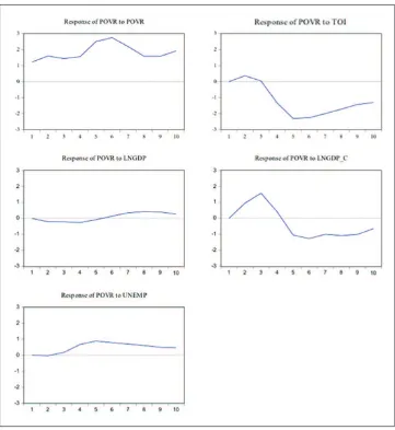
4.2. IRF
This analysis is to igure out the response of a variable when there is a shock in a variable and to see the effect of the shock duration of an endogenous variable which caused by other endogenous variable shock in a standard deviation. In this research, the run which is used to analyze the POVR response projected in the next
10 years. Figure 3, present the result of IRF simulation to measure the dynamical response of POVR to POVR, TOI, economic growth, income per capita, and OUR.
Based on Figure 4, it can be concluded that overall, the POVR would show positive response when there is one deviation change
on the variable of POVR. As an example, the POVR itself would pull up a positive response on the shock at 1.22%. The response
gets higher until the sixth year the POVR would give the positive
effect at 2.75%. On the next years the POVR would luctuate in
responding the shock which created by the POVR itself. During
10 years, the POVR would show the weakest response on the irst and third year, which only 1.22% and 1.44%. Until the end of the
period, the POVR would always show positive response to every shock caused by itself.
The shock of one deviation TOI would give effect on the raise of
POVR in the second and third each at 0.36% and 0.04%. On the Table 3: Johanssen’s co-integration test results
Hypothesized
At most 1* 0.962869 202.0898 47.85613 0.0000
At most 2* 0.810202 93.41042 29.79707 0.0000 At most 3* 0.619347 38.57112 15.49471 0.0000
At most 4* 0.183685 6.697507 3.841466 0.0097 *Denotes rejection of the hypothesis at the 5% level,**MacKinnon-Haug-Michelis
(1999) P values
Table 4: Short run and long run VECM estimation results Long run
*Indicates signiicance at 5% level, POVR: Poverty rate, TOI: Trade openness index,
next period, every shock on trade openness would give negative
effect on POVR. During 10 years, the POVR would show the weakest response on the third year, at 0.04%. On the other side, the POVR would show the biggest response on the ifth year, at −2.30%. Until the end of the period, the POVR would always
show the negative response to every shock produced by the TOI.
Response caused by the economic growth shock seen luctuating where on the irst ifth year the POVR showed negative response, while on the next year showed positive response. During the irst
5 year, the POVR would show the biggest negative response on
the fourth year, at 0.26%. On the sixth to the tenth year, the biggest
POVR response happened by one economic growth deviation
change on the eighth year, at 0.42%.
Differ with the shock by income per capita. On the irst 4 year, every
shock by one deviation income per capita, the POVR would show positive response, with the highest on the third year. However, after the fourth year, the POVR response caused by the shock of one deviation income per capita would receive negative response by
the POVR. The biggest response was on the sixth year, at −1.26%.
The shock of OUR at one deviation on the irst year would cause the POVR to give negative response, at −0.02%. On the next year
the POVR would show positive response when there was a one deviation change on the OUR. The POVR would show the biggest
response on the ifth year, at 0.88%.
The IRF showed that the shock on the TOI variable, economic growth, income per capita, and OUR could cause the POVR to
Figure 3: The impulse response of poverty rate results
decrease or increase. The shock of economic growth and OUR would cause the POVR to increase in the long run. The shock of TOI and income per capita would cause the POVR to decrease in the long run.
4.3. FEVD
FEVD is useful to explain the contribution of each variable to the shock caused by the observed main endogenous variable. The FEVD analysis on this research is to explain how big the contribution percentage of each shock of TOI variable, economic
growth, income per capita, and OUR in inluencing the POVR in Indonesia. The period used to explain the FEVD is 10 years. The
result of FEVD analysis can be seen on Figure 4.
Figure 4 shows that on the irst year, the luctuation of POVR
caused by the POVR itself at 100%. Started on the second year
to tenth year can be seen that other variables started to affect the POVR. On the second year, the POVR was still dominating at
79.08% while the variables that affect the POVR are income per capita at 17.45%, TOI at 2.58%, GDP at 0.84%, and UNEMP at 0.01%. On the third year, the POVR was still dominating at 62.87%, while other variable that gave major contribution in affecting the POVR is income per capita, at 34.48%. On the
next years, the income per capita contribution in affecting the POVR decreased, with the lowest contribution on the tenth year,
at 13.50%. The TOI during the irst 3 year had not showed big
contribution in affecting the POVR in Indonesia. However, on the fourth year to the tenth year, the TOI started to show big
contribution in affecting the POVR. The biggest inluence was on the ninth year, at 32.02%.
Figure 4 also shows that GDP does not show big contribution in affecting the POVR in Indonesia. The biggest contribution of GDP
variable in affecting the POVR was only 1.10%. As same as the UNEMP variable, which only contributed not more than 4.51%
to the POVR in Indonesia.
According to scientific journals and empirical fact revealed
on this research, it requires a commitment and strategy for the whole economic agents and stakeholders to create a fair trade
system. World Fair Trade Organization deines the fair trade as
a trade model based on the equal partnership through dialogue, transparency, and respect on each other. The purpose is to create fairness, sustainable development, protect the producers’ rights and marginal workers, and protect the environment from the damage by the exploration of economic activity.
Tjakrawerdaja et al., (2016) said that to realize the fair market, it requires; irst, the trade policy which focus on the fair market
institution with fair competition which consider the economic growth, the fair values, social interest, quality of life, and environmental sustainable development. Furthermore, it is hoped that every people in society has the same chance in striving and working, also the producers’ rights and the consumers are protected. Secondly, the development of fair competition, and prevent monopolistic market structure and other market structure which being distortion by the private sector, which harm the society. However, the essential resources and controlled the
human life should be owned by the country through national companies for the capital intensive industry, and cooperation for the labor intensive economic activity. Both national companies
and cooperation should be managed for the beneicial of entire
community in a country. Third, optimize role of the government in correcting the market failure through regulation, public service, subsidy, incentive, and disincentive. Fourth, develop the industrial policy, trade, and investment to increase the global competitiveness by opening the same accessibility to job opportunity and manage the people and the entire city through competitive advantage by using the comparative advantages, which are natural resources and human resources. It is called as Indonesia trade system based on Pancasila and 1945 Constitution of Indonesia, not the free trade competition.
5. CONCLUSION
Based on the research about the impact of trade openness on poverty in Indonesia, it can be concluded that the international
trade openness does not have the signiicant inluence to poverty in short run. However, in the long run, it has signiicant effect in
decreasing the POVR. The IRF analysis result concluded that the
POVR would show positive response in the irst 2 year, however,
on the next year, it would show negative response on every shock on the TOI variable. The negative response of POVR caused by the
shock on the trade openness variable would happen on the ifth year.
Based on the FEDV analysis result, the TOI during the irst
3 year would not give high contribution in affecting the POVR in Indonesia. However, on the fourth year until the tenth year, the trade openness would start to give high contribution in affecting the POVR. The biggest affect would be on the ninth year. To reduce the poverty through international trade, it requires an implementation of a fair trade system. So that all the economic agents could get
beneit, not become the predator for others.
REFERENCES
Abbott, K.W. (2003), Development Policy in the New Millennium and the Doha Development Round. Asian Development Bank. May, 2003. Available from: https://www.ssrn.com/abstract=431921, http://www. dx.doi.org/10.2139/ssrn.431921.
Amisano, G., Carlo, G. (1997), Topics in Structural VAR Econometrics.
Berlin, Heidelberg, Germany: Springer-Verlag.
Baudrillard, J.P. (2011), Masyarakat Konsumsi. Bantul: Kreasi Wacana. Besimi, F., Pugh, G., Adnett, N. (2006), The Monetary Transmission
Mechanism in Macedonia: Implications for Monetary Policy. Working Papers: Centre for Research on Emerging Economies Staffordshire University, 2, 1-34.
Chaudhry, I.S., Imran, F. (2013), Does trade liberalization reduce poverty
and inequality? Empirical evidence from Pakistan. Pakistan Journal of Commerce and Social Sciences, 7(3), 569-587.
Chen, S., Ravallion, M. (2007), Absolute Poverty Measures for the Developing World, 1981-2004. World Bank Policy Research
Working Paper No. 4211.
Dollar, D., Kraay, A. (2002), Growth is good for the poor. Journal of
Economic Growth, 7, 195-225.
Egunjobi, T.A. (2014), Poverty and unemployment paradox in Nigeria.
19(5), 106-116.
Enders, W. (2004), Applied Econometrics Time Series. 2nd ed. New York:
John Wiley & Sony Inc.
Engle, R.F., Granger, C.W.J. (1987), Cointegration and error correction representation, estimation and testing. Econometrica, 55, 251-276.
Fakih, M. (2002), Runtuhnya Teori Pembangunan dan Globalisasi. Yogyakarta: Pustaka Pelajar.
Firdaus, M. (2011), Aplikasi Ekonometrika untuk Data Panel dan Time
Series. Bogor: IPB Press.
Fischer, S. (2003), Globalization and its challenges. The American Economic Review, 93(2), 1-30.
Ginting, A.M. (2014), Trade balance development and its determining factors. Bulletin Ilmiah Litbang Perdagangan, 8(1), 51-72. Hameed, A., Nazir, A. (2004), Economic globalization and its impact on
poverty and inequality: Evidence from Pakistan. ECO Economic
Journal, 1, 1-21. Available from: http://www.eco.int/ftproot/ Publications/Journal/1/Article_TDB.pdf.
Harrison, A., editor. (2007), Introduction: Globalization and Poverty.
Chicago: University of Chicago Press and the National Bureau of Economic Research.
Harrison, A., Love, I., McMillan, M.S. (2004), Global capital lows and inancing constraints. Journal of Development Economics, 75(1), 269-301.
Huczynski, A., Buchanan, D. (2007), Organisational Behaviour: An.
Introductory Text. 6th ed. Harlow: FT, Prentice Hall.
Juanda, B., Junaidi. (2012), Ekonometrika Deret Waktu Teori dan Aplikasi. Bogor: IPB Press.
Lopez, J.H. (2004), Pro-Poor Growth: A Review of What We Know, (and of What We Don’t). World Bank. p1-20. Available from: http://www. eldis.org/vile/upload/1/document/0708/DOC17880.pdf.
McCulloch, N., Winters, L.A., Cirera, X. (2001), Trade Liberalization and Poverty: A Handbook. London: Centre for Economic Policy
Research and Department for International Development.
Mutascu, M., Fleischer, A. (2011), Economic growth and globalization in Romania. World Applied Science Journal, 12(10), 1691-1697. Myrdal, G. (1968), Asian Drama – An Inquiry into the Poverty of Nations.
New York: Pantheon.
Nissanke, M., Thorbecker, E. (2010), Globalization, poverty and inequality in Lation America: Findings from case studies. World Development, 38(6), 797-802.
Okungbowa, F.O.E., Eburajolo, C.O. (2014), Globalization and poverty rate in Nigeria: An empirical analysis. International Journal of
Humanities and Social Science, 4(11), 126-135.
Oyewale, I.O., Amusat, W.A. (2013), Impact of globalization on poverty
reduction in Nigeria. Interdisciplinary Journal of Contemporary Research in Business, 4(11), 475-484.
Ozcan, G., Kar, M. (2016), Does foreign trade liberalization reduce poverty in
Turkey? Journal of Economic and Social Development, 3(1), 157-173.
Ravallion, M. (2006), Looking beyond averages in the trade and poverty
debate. World Development, Elsevier, 34(8), 1374-1392.
Tjakrawerdaja, S., Purwandaya, B., Lenggono, P.S., Karim, M., Agusalim, L. (2016), Sistem Ekonomi Pancasila. Jakarta: Universitas
Trilogi.
Todaro, M.P., Smith, S.C. (2003), Pembangunan Ekonomi di Dunia Ketiga. Jilid 1. 8th ed. Jakarta: Erlangga.
Todaro, M.P., Smith, S.C. (2006), In: Barnadi, D., editor. Pembangunan
Ekonomi Haris Munandar, Intepreter. Translation from: Economic Development. 9th ed. Jakarta: Erlangga.
Twyford, P. (2003), Does Trade Liberalisation Exacerbate or Reduce Poverty? Trade and Globalisation in the Lead up to the Cancun Ministerial. Address to Council for International Development (CID) Trade Forum. Oxfam International. Landon.
Wirawan, I.M.T., Arka, S. (2015), Analisis pengaruh pendidikan, PDRB
per kapita, dan tingkat pengangguran terhadap jumlah penduduk miskin provinsi Bali. E-Jurnal Ekonomi Pembangunan Universitas