Current and Resistance
▲
These power lines transfer energy from the power company to homes and businesses. The energy is transferred at a very high voltage, possibly hundreds of thousands of volts in some cases. Despite the fact that this makes power lines very dangerous, the high voltage results in less loss of power due to resistance in the wires. (Telegraph Colour Library/FPG)Chapter 27
831
C H A P T E R O U T L I N E
27.1
Electric Current
27.2
Resistance
27.3
A Model for Electrical
Conduction
27.4
Resistance and Temperature
27.5
Superconductors
832
charges in equilibrium situations, or electrostatics. We now consider situations involving electric charges that are notin equilibrium. We use the term electric current, or simply current,to describe the rate of flow of charge through some region of space. Most prac-tical applications of electricity deal with electric currents. For example, the battery in a flashlight produces a current in the filament of the bulb when the switch is turned on. A variety of home appliances operate on alternating current. In these common situa-tions, current exists in a conductor, such as a copper wire. It also is possible for currents to exist outside a conductor. For instance, a beam of electrons in a television picture tube constitutes a current.
This chapter begins with the definition of current. A microscopic description of cur-rent is given, and some of the factors that contribute to the opposition to the flow of charge in conductors are discussed. A classical model is used to describe electrical con-duction in metals, and some of the limitations of this model are cited. We also define electrical resistance and introduce a new circuit element, the resistor. We conclude by discussing the rate at which energy is transferred to a device in an electric circuit.
27.1
Electric Current
In this section, we study the flow of electric charges through a piece of material. The amount of flow depends on the material through which the charges are passing and the potential difference across the material. Whenever there is a net flow of charge through some region, an electric currentis said to exist.
It is instructive to draw an analogy between water flow and current. In many localities it is common practice to install low-flow showerheads in homes as a water-conservation measure. We quantify the flow of water from these and similar devices by specifying the amount of water that emerges during a given time interval, which is often measured in liters per minute. On a grander scale, we can characterize a river current by describing the rate at which the water flows past a particular location. For example, the flow over the brink at Niagara Falls is maintained at rates between 1 400 m3/s and 2 800 m3/s.
There is also an analogy between thermal conduction and current. In Section 20.7, we discussed the flow of energy by heat through a sample of material. The rate of energy flow is determined by the material as well as the temperature difference across the material, as described by Equation 20.14.
To define current more precisely, suppose that charges are moving perpendicular to a surface of area A, as shown in Figure 27.1. (This area could be the cross-sectional area of a wire, for example.) The current is the rate at which charge flows through this
surface.If !Qis the amount of charge that passes through this area in a time interval
!t, the average currentIavis equal to the charge that passes through Aper unit time:
(27.1) Iav"
∆Q ∆t
A
I
+
+
+ +
+
If the rate at which charge flows varies in time, then the current varies in time; we define the instantaneous currentIas the differential limit of average current:
(27.2)
The SI unit of current is the ampere (A):
(27.3)
That is, 1 A of current is equivalent to 1 C of charge passing through the surface area in 1 s.
The charges passing through the surface in Figure 27.1 can be positive or negative, or both. It is conventional to assign to the current the same direction as the flow
of positive charge.In electrical conductors, such as copper or aluminum, the current
is due to the motion of negatively charged electrons. Therefore, when we speak of current in an ordinary conductor, the direction of the current is opposite the
direction of flow of electrons. However, if we are considering a beam of positively
charged protons in an accelerator, the current is in the direction of motion of the protons. In some cases—such as those involving gases and electrolytes, for instance— the current is the result of the flow of both positive and negative charges.
If the ends of a conducting wire are connected to form a loop, all points on the loop are at the same electric potential, and hence the electric field is zero within and at the surface of the conductor. Because the electric field is zero, there is no net transport of charge through the wire, and therefore there is no current. However, if the ends of the conducting wire are connected to a battery, all points on the loop are not at the same potential. The battery sets up a potential difference between the ends of the loop, creating an electric field within the wire. The electric field exerts forces on the conduction electrons in the wire, causing them to move in the wire, thus creating a current.
It is common to refer to a moving charge (positive or negative) as a mobile charge
carrier.For example, the mobile charge carriers in a metal are electrons.
Microscopic Model of Current
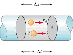
We can relate current to the motion of the charge carriers by describing a microscopic model of conduction in a metal. Consider the current in a conductor of cross-sectional area A (Fig. 27.2). The volume of a section of the conductor of length !x(the gray region shown in Fig. 27.2) is A!x. If n represents the number of mobile charge carriers per unit volume (in other words, the charge carrier density), the number of carriers in the gray section is nA!x. Therefore, the total charge !Qin this section is
!Q"number of carriers in section#charge per carrier"(nA!x)q
where qis the charge on each carrier. If the carriers move with a speed vd, the displace-ment they experience in the xdirection in a time interval !t is !x"vd !t. Let us choose !t to be the time interval required for the charges in the cylinder to move through a displacement whose magnitude is equal to the length of the cylinder. This time interval is also that required for all of the charges in the cylinder to pass through the circular area at one end. With this choice, we can write !Qin the form
!Q"(nAvd!t)q
If we divide both sides of this equation by !t, we see that the average current in the conductor is
(27.4) Iav"
∆Q
∆t "nqvdA 1 A" 1 C
1 s I ! dQ
dt
S E C T I O N 27. 1 • Electric Current 833
▲
PITFALL PREVENTION
27.1
“Current Flow” Is
Redundant
The phrase current flow is com-monly used, although it is strictly incorrect, because current is a flow (of charge). This is similar to the phrase heat transfer, which is also redundant because heat is
a transfer (of energy). We will avoid this phrase and speak of
flow of charge or charge flow. Electric current
∆x
A q
vd
vd∆t
Figure 27.2 A section of a uniform conductor of cross-sectional area A. The mobile charge carriers move with a speed vd, and the displace-ment they experience in the x
direction in a time interval !tis !x"vd!t. If we choose !tto be the time interval during which the charges are displaced, on the average, by the length of the cylinder, the number of carriers in the section of length !xis nAvd!t, where nis the number of carriers per unit volume.
The speed of the charge carriers vdis an average speed called the drift speed.To understand the meaning of drift speed, consider a conductor in which the charge car-riers are free electrons. If the conductor is isolated—that is, the potential difference across it is zero—then these electrons undergo random motion that is analogous to the motion of gas molecules. As we discussed earlier, when a potential difference is applied across the conductor (for example, by means of a battery), an electric field is set up in the conductor; this field exerts an electric force on the electrons, producing a current. However, the electrons do not move in straight lines along the conductor. Instead, they collide repeatedly with the metal atoms, and their resultant motion is complicated and zigzag (Fig. 27.3). Despite the collisions, the electrons move slowly along the conduc-tor (in a direction opposite that of E) at the drift velocity vd.
We can think of the atom–electron collisions in a conductor as an effective internal friction (or drag force) similar to that experienced by the molecules of a liquid flowing through a pipe stuffed with steel wool. The energy transferred from the electrons to the metal atoms during collisions causes an increase in the vibrational energy of the atoms and a corresponding increase in the temperature of the conductor.
Figure 27.3 A schematic representation of the zigzag motion of an electron in a conductor. The changes in direction are the result of collisions between the electron and atoms in the conductor. Note that the net motion of the electron is opposite the direction of the electric field. Because of the acceleration of the charge carriers due to the electric force, the paths are actually parabolic. However, the drift speed is much smaller than the average speed, so the parabolic shape is not visible on this scale.
Quick Quiz 27.1
Consider positive and negative charges movinghorizon-tally through the four regions shown in Figure 27.4. Rank the current in these four regions, from lowest to highest.
Quick Quiz 27.2
Electric charge is conserved. As a consequence, when currentarrives at a junction of wires, the charges can take either of two paths out of the junction and the numerical sum of the currents in the two paths equals the current that entered the junction. Thus, current is (a) a vector (b) a scalar (c) neither a vector nor a scalar. vd
E –
Figure 27.4 (Quick Quiz 27.1) Charges move through four regions. (a)
Example 27.1 Drift Speed in a Copper Wire
The 12-gauge copper wire in a typical residential building has a cross-sectional area of 3.31#10$6m2. If it carries a current of 10.0 A, what is the drift speed of the electrons? Assume that each copper atom contributes one free electron to the current. The density of copper is 8.95 g/cm3.
Solution From the periodic table of the elements in Appendix C, we find that the molar mass of copper is 63.5 g/mol. Recall that 1 mol of any substance contains Avogadro’s number of atoms (6.02#1023). Knowing the density of copper, we can calculate the volume occupied by 63.5 g ("1 mol) of copper:
Because each copper atom contributes one free electron to the current, we have
V" m % "
63.5 g
8.95 g/cm3 "7.09 cm3
From Equation 27.4, we find that the drift speed is
Example 27.1 shows that typical drift speeds are very low. For instance, electrons traveling with a speed of 2.22#10$4m/s would take about 75 min to travel 1 m! In
view of this, you might wonder why a light turns on almost instantaneously when a switch is thrown. In a conductor, changes in the electric field that drives the free electrons travel through the conductor with a speed close to that of light. Thus, when you flip on a light switch, electrons already in the filament of the lightbulb experience electric forces and begin moving after a time interval on the order of nanoseconds.
27.2
Resistance
In Chapter 24 we found that the electric field inside a conductor is zero. However, this statement is true only if the conductor is in static equilibrium. The purpose of this section is to describe what happens when the charges in the conductor are not in equi-librium, in which case there is an electric field in the conductor.
Consider a conductor of cross-sectional area Acarrying a current I. The current
densityJin the conductor is defined as the current per unit area. Because the current
I"nqvdA, the current density is
(27.5)
where Jhas SI units of A/m2. This expression is valid only if the current density is uni-form and only if the surface of cross-sectional area Ais perpendicular to the direction of the current. In general, current density is a vector quantity:
(27.6)
From this equation, we see that current density is in the direction of charge motion for positive charge carriers and opposite the direction of motion for negative charge carriers.
A current density J and an electric field E are established in a conductor
whenever a potential difference is maintained across the conductor. In some
materials, the current density is proportional to the electric field:
J"&E (27.7)
where the constant of proportionality &is called the conductivityof the conductor.1 Materials that obey Equation 27.7 are said to follow Ohm’s law,named after Georg Simon Ohm (1789–1854). More specifically, Ohm’s law states that
J"nqvd J ! I
A "nqvd
S E C T I O N 27. 2 • Resistance 835
▲
PITFALL PREVENTION
27.2
Electrons Are
Available Everywhere
Electrons do not have to travel from the light switch to the light in order for the light to operate. Electrons already in the filament of the lightbulb move in response to the electric field set up by the battery. Notice also that a battery does not provide electrons to the circuit. It establishes the electric field that exerts a force on electrons already in the wires and elements of the circuit.
Current density
for many materials (including most metals), the ratio of the current density to the electric field is a constant &that is independent of the electric field producing the current.
Materials that obey Ohm’s law and hence demonstrate this simple relationship between Eand Jare said to be ohmic.Experimentally, however, it is found that not all materials have this property. Materials and devices that do not obey Ohm’s law are said to be nonohmic.Ohm’s law is not a fundamental law of nature but rather an empirical relationship valid only for certain materials.
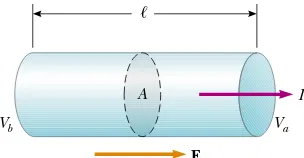
We can obtain an equation useful in practical applications by considering a segment of straight wire of uniform cross-sectional area Aand length !, as shown in
Georg Simon Ohm
German physicist (1789–1854)
Figure 27.5. A potential difference !V"Vb$Vais maintained across the wire, creat-ing in the wire an electric field and a current. If the field is assumed to be uniform, the potential difference is related to the field through the relationship2
!V"E!
Therefore, we can express the magnitude of the current density in the wire as
Because J"I/A, we can write the potential difference as
The quantity R"!/&Ais called the resistanceof the conductor. We can define the resistance as the ratio of the potential difference across a conductor to the current in the conductor:
(27.8)
We will use this equation over and over again when studying electric circuits. From this result we see that resistance has SI units of volts per ampere. One volt per ampere is defined to be one ohm('):
(27.9)
This expression shows that if a potential difference of 1 V across a conductor causes a current of 1 A, the resistance of the conductor is 1'. For example, if an electrical appliance connected to a 120-V source of potential difference carries a current of 6 A, its resistance is 20'.
The inverse of conductivity is resistivity3%:
(27.10)
where % has the units ohm-meters (' (m). Because R"!/&A, we can express the resistance of a uniform block of material along the length !as
(27.11) R"% !
A % " 1
& 1 '! 1 V
1 A R ! ∆V
I ∆V" !
& J"
"
!&A
#
I"RI J"&E"&∆V !
!
E
Vb Va
I A
Resistivity is the inverse of conductivity
Resistance of a uniform material along the length !
Figure 27.5A uniform conductor of length !and cross-sectional area A. A potential difference !V"Vb$Vamaintained across the conductor sets up an electric field E, and this field produces a current Ithat is proportional to the potential difference.
2 This result follows from the definition of potential difference:
3 Do not confuse resistivity %with mass density or charge density, for which the same symbol is used.
Vb$Va" $
$
ba E(ds"E
$
!
0
dx"E!
▲
PITFALL PREVENTION
27.3
We’ve Seen
Something Like
Equation 27.8 Before
In Chapter 5, we introduced Newton’s second law, )F"ma, for a net force on an object of mass m. This can be written as
In that chapter, we defined mass as resistance to a change in motion in response to an external force. Mass as resistance to changes in motion is analogous to electrical resistance to charge flow, and Equation 27.8 is analogous to the form of Newton’s second law shown here.
m"
%
Fa
▲
PITFALL PREVENTION
27.4
Equation 27.8 Is Not
Ohm’s Law
Every ohmic material has a characteristic resistivity that depends on the properties of the material and on temperature. Additionally, as you can see from Equation 27.11, the resistance of a sample depends on geometry as well as on resistivity. Table 27.1 gives the resistivities of a variety of materials at 20°C. Note the enormous range, from very low values for good conductors such as copper and silver, to very high values for good insulators such as glass and rubber. An ideal conductor would have zero resistivity, and an ideal insulator would have infinite resistivity.
Equation 27.11 shows that the resistance of a given cylindrical conductor such as a wire is proportional to its length and inversely proportional to its cross-sectional area. If the length of a wire is doubled, then its resistance doubles. If its cross-sectional area is doubled, then its resistance decreases by one half. The situation is analogous to the flow of a liquid through a pipe. As the pipe’s length is increased, the resistance to flow increases. As the pipe’s cross-sectional area is increased, more liquid crosses a given cross section of the pipe per unit time interval. Thus, more liquid flows for the same pressure differential applied to the pipe, and the resistance to flow decreases.
S E C T I O N 27. 2 • Resistance 837
▲
PITFALL PREVENTION
27.5
Resistance and
Resistivity
Resistivity is property of a sub-stance, while resistance is a prop-erty of an object. We have seen similar pairs of variables before. For example, density is a prop-erty of a substance, while mass is a property of an object. Equation 27.11 relates resistance to resistiv-ity, and we have seen a previous equation (Equation 1.1) which relates mass to density.
Temperature
Material Resistivitya(' (m) Coefficientb![(!C)$1]
Silver 1.59#10$8 3.8#10$3
Copper 1.7#10$8 3.9#10$3
Gold 2.44#10$8 3.4#10$3
Aluminum 2.82#10$8 3.9#10$3
Tungsten 5.6#10$8 4.5#10$3
Iron 10#10$8 5.0#10$3
Platinum 11#10$8 3.92#10$3
Lead 22#10$8 3.9#10$3
Nichromec 1.50#10$6 0.4#10$3
Carbon 3.5#10$5 $0.5#10$3
Germanium 0.46 $48#10$3
Silicon 640 $75#10$3
Glass 1010to 1014
Hard rubber &1013
Sulfur 1015
Quartz (fused) 75#1016
Resistivities and Temperature Coefficients of Resistivity for Various Materials
Table 27.1
a All values at 20°C.
b See Section 27.4.
c A nickel–chromium alloy commonly used in heating elements.
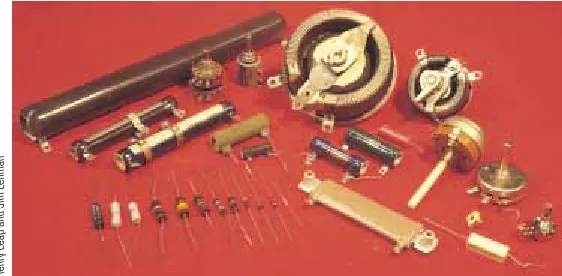
An assortment of resistors used in electrical circuits.
Most electric circuits use circuit elements called resistors to control the current level in the various parts of the circuit. Two common types of resistors are the
composi-tion resistor,which contains carbon, and the wire-wound resistor,which consists of a coil of
wire. Values of resistors in ohms are normally indicated by color-coding, as shown in Figure 27.6 and Table 27.2.
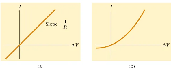
Ohmic materials and devices have a linear current–potential difference relation-ship over a broad range of applied potential differences (Fig. 27.7a). The slope of the I-versus-!Vcurve in the linear region yields a value for 1/R. Nonohmic materials have a nonlinear current–potential difference relationship. One common semiconducting device that has nonlinear I-versus-!V characteristics is the junction diode (Fig. 27.7b). The resistance of this device is low for currents in one direction (positive !V) and high for currents in the reverse direction (negative !V). In fact, most modern electronic devices, such as transistors, have nonlinear current–potential difference relationships; their proper operation depends on the particular way in which they violate Ohm’s law.
Color Number Multiplier Tolerance
Black 0 1
Brown 1 101
Red 2 102
Orange 3 103
Yellow 4 104
Green 5 105
Blue 6 106
Violet 7 107
Gray 8 108
White 9 109
Gold 10$1 5%
Silver 10$2 10%
Colorless 20%
Color Coding for Resistors
Table 27.2
(a) I
Slope = 1 R
!V
(b) I
!V
Figure 27.7 (a) The current–potential difference curve for an ohmic material. The curve is linear, and the slope is equal to the inverse of the resistance of the conductor. (b) A nonlinear current–potential difference curve for a junction diode. This device does not obey Ohm’s law.
Figure 27.6 The colored bands on a resistor represent a code for determining resistance. The first two colors give the first two digits in the resistance value. The third color represents the power of ten for the multiplier of the resistance value. The last color is the tolerance of the resistance value. As an example, the four colors on the circled resistors are red ("2), black ("0), orange ("103), and gold ("5%), and so the
resistance value is 20#103' "20 k'with a tolerance value of 5%"1 k'.
(The values for the colors are from Table 27.2.)
SuperStock
Quick Quiz 27.3
Suppose that a current-carrying ohmic metal wire has aS E C T I O N 27. 2 • Resistance 839
unit length vary along the wire as the area becomes smaller? (a) The drift velocity and resistance both increase. (b) The drift velocity and resistance both decrease. (c) The drift velocity increases and the resistance decreases. (d) The drift velocity decreases and the resistance increases.
Quick Quiz 27.4
A cylindrical wire has a radius rand length !. If both rand !are doubled, the resistance of the wire (a) increases (b) decreases (c) remains the same.
Quick Quiz 27.5
In Figure 27.7b, as the applied voltage increases, theresis-tance of the diode (a) increases (b) decreases (c) remains the same.
Example 27.2 The Resistance of a Conductor
Example 27.3 The Resistance of Nichrome Wire
Example 27.4 The Radial Resistance of a Coaxial Cable
Calculate the resistance of an aluminum cylinder that has a length of 10.0 cm and a cross-sectional area of 2.00#10$4m2. Repeat the calculation for a cylinder of the same dimensions and made of glass having a resistivity of 3.0#1010' (m.
Solution From Equation 27.11 and Table 27.1, we can cal-culate the resistance of the aluminum cylinder as follows:
1.41#10$5 '
"
R"% !
A "(2.82#10
$8' (m)
"
0.100 m2.00#10$4 m2
#
Similarly, for glass we find that
As you might guess from the large difference in resistivities, the resistances of identically shaped cylinders of aluminum and glass differ widely. The resistance of the glass cylinder is 18 orders of magnitude greater than that of the aluminum cylinder.
1.5#1013'
"
R"% !
A "(3.0#10
10' (m)
"
0.100 m2.00#10$4 m2
#
(A) Calculate the resistance per unit length of a 22-gauge Nichrome wire, which has a radius of 0.321 mm.
Solution The cross-sectional area of this wire is
The resistivity of Nichrome is 1.5#10$6' (m (see Table 27.1). Thus, we can use Equation 27.11 to find the resistance per unit length:
(B) If a potential difference of 10 V is maintained across a 1.0-m length of the Nichrome wire, what is the current in the wire?
4.6 '/m R
! " %
A "
1.5#10$6' (m 3.24#10$7 m2 "
A"*r2"*(0.321#10$3 m)2"3.24#10$7 m2
Solution Because a 1.0-m length of this wire has a resis-tance of 4.6', Equation 27.8 gives
Note from Table 27.1 that the resistivity of Nichrome wire is about 100 times that of copper. A copper wire of the same radius would have a resistance per unit length of only 0.052 '/m. A 1.0-m length of copper wire of the same radius would carry the same current (2.2 A) with an applied potential difference of only 0.11 V.
Because of its high resistivity and its resistance to oxidation, Nichrome is often used for heating elements in toasters, irons, and electric heaters.
2.2 A I" ∆V
R " 10 V 4.6 ' "
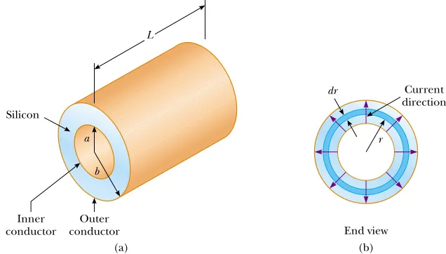
silicon, in the radial direction, is unwanted. (The cable is designed to conduct current along its length—this is not the current we are considering here.) The radius of the inner conductor is a"0.500 cm, the radius of the outer one is b"1.75 cm, and the length is L"15.0 cm. Coaxial cables are used extensively for cable television and
other electronic applications. A coaxial cable consists of two concentric cylindrical conductors. The region between the conductors is completely filled with silicon, as shown in Figure 27.8a, and current leakage through the
Interactive
Figure 27.8(Example 27.4) A coaxial cable. (a) Silicon fills the gap between the two conductors. (b) End view, showing current leakage.
Calculate the resistance of the silicon between the two conductors.
Solution Conceptualize by imagining two currents, as suggested in the text of the problem. The desired current is along the cable, carried within the conductors. The undesired current corresponds to charge leakage through the silicon and its direction is radial. Because we know the resistivity and the geometry of the silicon, we categorize this as a problem in which we find the resistance of the silicon from these parameters, using Equation 27.11. Because the area through which the charges pass depends on the radial position, we must use integral calculus to determine the answer.
To analyze the problem, we divide the silicon into con-centric elements of infinitesimal thickness dr (Fig. 27.8b). We start by using the differential form of Equation 27.11, replacing ! with r for the distance variable: dR"%dr/A, where dR is the resistance of an element of silicon of thickness drand surface area A. In this example, we take as our representative concentric element a hollow silicon cylin-der of radius r, thickness dr, and length L, as in Figure 27.8. Any charge that passes from the inner conductor to the outer one must pass radially through this concentric ele-ment, and the area through which this charge passes is A"2*rL. (This is the curved surface area—circumference multiplied by length—of our hollow silicon cylinder of thickness dr.) Hence, we can write the resistance of our hollow cylinder of silicon as
Because we wish to know the total resistance across the entire thickness of the silicon, we must integrate this expres-sion from r"ato r"b:
Substituting in the values given, and using % "640' (m for silicon, we obtain
To finalize this problem, let us compare this resistance to that of the inner conductor of the cable along the 15.0-cm length. Assuming that the conductor is made of copper, we have
This resistance is much smaller than the radial resistance. As a consequence, almost all of the current corresponds to charge moving along the length of the cable, with a very small fraction leaking in the radial direction.
What If? Suppose the coaxial cable is enlarged to twice the overall diameter with two possibilities: (1) the ratio b/a is held fixed, or (2) the difference b"ais held fixed. For which possibility does the leakage current between the inner and outer conductors increase when the voltage is applied between the two conductors?
27.3
A Model for Electrical Conduction
In this section we describe a classical model of electrical conduction in metals that was first proposed by Paul Drude (1863–1906) in 1900. This model leads to Ohm’s law and shows that resistivity can be related to the motion of electrons in metals. Although the Drude model described here does have limitations, it nevertheless introduces concepts that are still applied in more elaborate treatments.
Consider a conductor as a regular array of atoms plus a collection of free electrons, which are sometimes called conduction electrons. The conduction electrons, although bound to their respective atoms when the atoms are not part of a solid, gain mobility when the free atoms condense into a solid. In the absence of an electric field, the conduc-tion electrons move in random direcconduc-tions through the conductor with average speeds on the order of 106m/s. The situation is similar to the motion of gas molecules confined in a
vessel. In fact, some scientists refer to conduction electrons in a metal as an electron gas. There is no current in the conductor in the absence of an electric field because the drift velocity of the free electrons is zero. That is, on the average, just as many electrons move in one direction as in the opposite direction, and so there is no net flow of charge.
This situation changes when an electric field is applied. Now, in addition to under-going the random motion just described, the free electrons drift slowly in a direction opposite that of the electric field, with an average drift speed vdthat is much smaller (typically 10$4m/s) than their average speed between collisions (typically 106m/s).
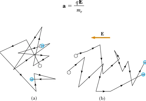
Figure 27.9 provides a crude description of the motion of free electrons in a conductor. In the absence of an electric field, there is no net displacement after many collisions (Fig. 27.9a). An electric field Emodifies the random motion and causes the electrons to drift in a direction opposite that of E(Fig. 27.9b).
In our model, we assume that the motion of an electron after a collision is indepen-dent of its motion before the collision. We also assume that the excess energy acquired by the electrons in the electric field is lost to the atoms of the conductor when the electrons and atoms collide. The energy given up to the atoms increases their vibra-tional energy, and this causes the temperature of the conductor to increase. The tem-perature increase of a conductor due to resistance is utilized in electric toasters and other familiar appliances.
We are now in a position to derive an expression for the drift velocity. When a free electron of mass me and charge q(" $e) is subjected to an electric field E, it experiences a force F"qE. Because this force is related to the acceleration of the electron through Newton’s second law, F"mea, we conclude that the acceleration of the electron is
(27.12)
a" qE me
S E C T I O N 27. 3 • A Model for Electrical Conduction 841
At the Active Figures link at http://www.pse6.com,you can adjust the electric field to see the resulting effect on the motion of an electron.
Active Figure 27.9 (a) A schematic diagram of the random motion of two charge carriers in a conductor in the absence of an electric field. The drift velocity is zero. (b) The motion of the charge carriers in a conductor in the presence of an electric field. Note that the random motion is modified by the field, and the charge carriers have a drift velocity.
(a) –
– ––
–
– –
– E
This acceleration, which occurs for only a short time interval between collisions, enables the electron to acquire a small drift velocity. If viis the electron’s initial velocity the instant after a collision (which occurs at a time that we define as t"0), then the velocity of the electron at time t(at which the next collision occurs) is
(27.13)
We now take the average value of vfover all possible collision times tand all possible values of vi. If we assume that the initial velocities are randomly distributed over all possible values, we see that the average value of viis zero. The term (qE/me)tis the velocity change of the electron due to the electric field during one trip between atoms. The average value of the second term of Equation 27.13 is (qE/me)+, where + is the average time interval between successive collisions. Because the average value of vfis equal to the drift velocity, we have
(27.14)
We can relate this expression for drift velocity to the current in the conductor. Substituting Equation 27.14 into Equation 27.6, we find that the magnitude of the current density is
(27.15)
where nis the number of charge carriers per unit volume. Comparing this expression with Ohm’s law, J"&E, we obtain the following relationships for conductivity and resistivity of a conductor:
(27.16)
(27.17)
According to this classical model, conductivity and resistivity do not depend on the strength of the electric field. This feature is characteristic of a conductor obeying Ohm’s law.
The average time interval + between collisions is related to the average distance between collisions !(that is, the mean free path; see Section 21.7) and the average speed
through the expression
(27.18) + " !
v v
% " 1 & "
me nq2+ & " nq
2+
me J"nqvd"
nq2E me
+
vf"vd"
qE
me +
vf"vi,at"vi,
qE
me t
Drift velocity in terms of microscopic quantities
Current density in terms of microscopic quantities
Conductivity in terms of micro-scopic quantities
Resistivity in terms of micro-scopic quantities
Example 27.5 Electron Collisions in a Wire
(A) Using the data and results from Example 27.1 and the classical model of electron conduction, estimate the average time interval between collisions for electrons in household copper wiring.
Solution From Equation 27.17, we see that
where % "1.7#10$8' (m for copper and the carrier den-sity is n"8.49#1028electrons/m3for the wire described
+ " me
nq2%
in Example 27.1. Substitution of these values into the expression above gives
2.5#10$14 s
"
+ " 9.11#10
$31 kg
(8.49#1028 m$3)(1.6#10$19 C)2 (1.7#10$8' (m )
27.4
Resistance and Temperature
Over a limited temperature range, the resistivity of a conductor varies approximately linearly with temperature according to the expression
(27.19)
where %is the resistivity at some temperature T(in degrees Celsius), %0is the resistivity at some reference temperature T0(usually taken to be 20°C), and -is the
tempera-ture coefficient of resistivity. From Equation 27.19, we see that the temperature
coefficient of resistivity can be expressed as
(27.20)
where !% " % $ %0is the change in resistivity in the temperature interval !T"T$T0.
The temperature coefficients of resistivity for various materials are given in Table 27.1. Note that the unit for -is degrees Celsius$1[(°C)$1]. Because resistance is proportional to resistivity (Eq. 27.11), we can write the variation of resistance as
(27.21)
Use of this property enables us to make precise temperature measurements, as shown in Example 27.6.
R"R0[1,-(T$T0)] - " 1
%0 ∆% ∆T % " %0[1,-(T$T0)]
S E C T I O N 27. 4 • Resistance and Temperature 843
Quick Quiz 27.6
When does a lightbulb carry more current: (a) just after itis turned on and the glow of the metal filament is increasing, or (b) after it has been on for a few milliseconds and the glow is steady?
which is equivalent to 40 nm (compared with atomic spacings of about 0.2 nm). Thus, although the time interval between collisions is very short, an electron in the wire travels about 200 atomic spacings between collisions. Solution From Equation 27.18,
4.0#10$8 m
"
!"v+ "(1.6#106 m/s)(2.5#10$14 s)
Example 27.6 A Platinum Resistance Thermometer
A resistance thermometer, which measures temperature by measuring the change in resistance of a conductor, is made from platinum and has a resistance of 50.0' at 20.0°C. When immersed in a vessel containing melting indium, its resistance increases to 76.8'. Calculate the melting point of the indium.
Solution Solving Equation 27.21 for !T and using the
-value for platinum given in Table 27.1, we obtain
Because T0"20.0°C, we find that T, the temperature of the
melting indium sample, is 157.C.
"137.C ∆T" R$R0
-R0
" 76.8 ' $50.0 '
[3.92#10$3(.C)$1](50.0 ')
For metals like copper, resistivity is nearly proportional to temperature, as shown in Figure 27.10. However, a nonlinear region always exists at very low temperatures, and the resistivity usually reaches some finite value as the temperature approaches absolute zero. This residual resistivity near absolute zero is caused primarily by the
Variation of #with temperature
collision of electrons with impurities and imperfections in the metal. In contrast, high-temperature resistivity (the linear region) is predominantly characterized by collisions between electrons and metal atoms.
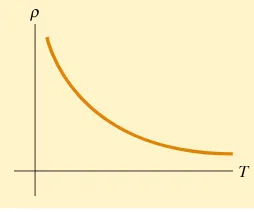
Notice that three of the -values in Table 27.1 are negative; this indicates that the resistivity of these materials decreases with increasing temperature (Fig. 27.11), which is indicative of a class of materials called semiconductors. This behavior is due to an increase in the density of charge carriers at higher temperatures.
Because the charge carriers in a semiconductor are often associated with impurity atoms, the resistivity of these materials is very sensitive to the type and concentration of such impurities. We shall return to the study of semiconductors in Chapter 43.
27.5
Superconductors
There is a class of metals and compounds whose resistance decreases to zero when they are below a certain temperature Tc, known as the critical temperature. These materials are known as superconductors. The resistance–temperature graph for a superconductor follows that of a normal metal at temperatures above Tc(Fig. 27.12). When the temperature is at or below Tc, the resistivity drops suddenly to zero. This phenomenon was discovered in 1911 by the Dutch physicist Heike Kamerlingh-Onnes (1853–1926) as he worked with mercury, which is a superconductor below 4.2 K. Recent measurements have shown that the resistivities of superconductors below their Tcvalues are less than 4#10$25' (m—around 1017times smaller than the resistivity of copper and in practice considered to be zero.
Today thousands of superconductors are known, and as Table 27.3 illustrates, the critical temperatures of recently discovered superconductors are substantially higher than initially thought possible. Two kinds of superconductors are recognized. The more recently identified ones are essentially ceramics with high critical temperatures, whereas superconducting materials such as those observed by Kamerlingh-Onnes are metals. If a room-temperature superconductor is ever identified, its impact on technology could be tremendous.
The value of Tc is sensitive to chemical composition, pressure, and molecular structure. It is interesting to note that copper, silver, and gold, which are excellent conductors, do not exhibit superconductivity.
Material Tc(K)
HgBa2Ca2Cu3O8 134
Tl–Ba–Ca–Cu–O 125
Bi–Sr–Ca–Cu–O 105
YBa2Cu3O7 92
Nb3Ge 23.2
Nb3Sn 18.05
Nb 9.46
Pb 7.18
Hg 4.15
Sn 3.72
Al 1.19
Zn 0.88
Critical Temperatures for Various Superconductors
Table 27.3
Figure 27.11 Resistivity versus temperature for a pure
semiconductor, such as silicon or germanium.
Figure 27.12 Resistance versus temperature for a sample of mercury (Hg). The graph follows that of a normal metal above the critical temperature Tc. The resistance drops to zero at Tc, which is 4.2 K for mercury. T
ρ
0
T ρ0
0 ρ
ρ
Figure 27.10 Resistivity versus temperature for a metal such as copper. The curve is linear over a wide range of temperatures, and %
increases with increasing temperature. As Tapproaches absolute zero (inset), the resistivity approaches a finite value %0.
ρ
T
0.10
0.05
4.4 4.2
4.0
T(K) 0.15
R(Ω)
Tc
One of the truly remarkable features of superconductors is that once a current is set up in them, it persists without any applied potential difference(because R"0). Steady currents have been observed to persist in superconducting loops for several years with no apparent decay!
An important and useful application of superconductivity is in the development of superconducting magnets, in which the magnitudes of the magnetic field are about ten times greater than those produced by the best normal electromagnets. Such superconducting magnets are being considered as a means of storing energy. Superconducting magnets are currently used in medical magnetic resonance imaging (MRI) units, which produce high-quality images of internal organs without the need for excessive exposure of patients to x-rays or other harmful radiation.
For further information on superconductivity, see Section 43.8.
27.6
Electrical Power
If a battery is used to establish an electric current in a conductor, there is a continuous transformation of chemical energy in the battery to kinetic energy of the electrons to internal energy in the conductor, resulting in an increase in the temperature of the conductor.
In typical electric circuits, energy is transferred from a source such as a battery, to some device, such as a lightbulb or a radio receiver. Let us determine an expression that will allow us to calculate the rate of this energy transfer. First, consider the simple circuit in Figure 27.13, where we imagine energy is being delivered to a resistor. (Resistors are designated by the circuit symbol .) Because the connecting wires also have resistance, some energy is delivered to the wires and some energy to the resistor. Unless noted otherwise, we shall assume that the resistance of the wires is so small compared to the resistance of the circuit element that we ignore the energy delivered to the wires.
Imagine following a positive quantity of charge Qthat is moving clockwise around the circuit in Figure 27.13 from point athrough the battery and resistor back to point a. We identify the entire circuit as our system. As the charge moves from ato bthrough the battery, the electric potential energy of the system increases by an amount Q!Vwhile the chemical potential energy in the battery decreasesby the same amount. (Recall from Eq. 25.9 that !U"q!V.) However, as the charge moves from c to d through the resistor, the system losesthis electric potential energy during collisions of electrons with atoms in the resistor. In this process, the energy is transformed to internal energy corresponding to increased vibrational motion of the atoms in the resistor. Because we have neglected the resistance of the interconnecting wires, no energy transformation occurs for paths bcand da.When the charge returns to point a, the net result is that some of the chemical energy in the battery has been delivered to the resistor and resides in the resistor as internal energy associated with molecular vibration.
The resistor is normally in contact with air, so its increased temperature will result in a transfer of energy by heat into the air. In addition, the resistor emits thermal
S E C T I O N 27. 6 • Electrical Power 845
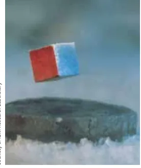
A small permanent magnet levitated above a disk of the superconductor YBa2Cu3O7,which
is at 77 K.
Courtesy of IBM Research Laboratory
At the Active Figures link at http://www.pse6.com,you can adjust the battery voltage and the resistance to see the resulting current in the circuit and power delivered to the resistor.
Active Figure 27.13 A circuit consisting of a resistor of
resistance Rand a battery having a potential difference !Vacross its terminals. Positive charge flows in the clockwise direction. b
a
c
d R I
∆V +
–
▲
PITFALL PREVENTION
27.6
Misconceptions
About Current
radiation, representing another means of escape for the energy. After some time interval has passed, the resistor reaches a constant temperature, at which time the input of energy from the battery is balanced by the output of energy by heat and radiation. Some electrical devices include heat sinks4connected to parts of the circuit to prevent these parts from reaching dangerously high temperatures. These are pieces of metal with many fins. The high thermal conductivity of the metal provides a rapid transfer of energy by heat away from the hot component, while the large number of fins provides a large surface area in contact with the air, so that energy can transfer by radiation and into the air by heat at a high rate.
Let us consider now the rate at which the system loses electric potential energy as the charge Qpasses through the resistor:
where Iis the current in the circuit. The system regains this potential energy when the charge passes through the battery, at the expense of chemical energy in the battery. The rate at which the system loses potential energy as the charge passes through the resistor is equal to the rate at which the system gains internal energy in the resistor. Thus, the power ", representing the rate at which energy is delivered to the resistor, is
(27.22)
We derived this result by considering a battery delivering energy to a resistor. However, Equation 27.22 can be used to calculate the power delivered by a voltage source to any device carrying a current Iand having a potential difference !Vbetween its terminals. Using Equation 27.22 and the fact that !V"IRfor a resistor, we can express the power delivered to the resistor in the alternative forms
(27.23)
When Iis expressed in amperes, !Vin volts, and Rin ohms, the SI unit of power is the watt, as it was in Chapter 7 in our discussion of mechanical power. The process by which power is lost as internal energy in a conductor of resistance Ris often called joule heating5; this transformation is also often referred to as an I2Rloss.
When transporting energy by electricity through power lines, such as those shown in the opening photograph for this chapter, we cannot make the simplifying assumption that the lines have zero resistance. Real power lines do indeed have resistance, and power is delivered to the resistance of these wires. Utility companies seek to minimize the power transformed to internal energy in the lines and maxi-mize the energy delivered to the consumer. Because ""I!V, the same amount of power can be transported either at high currents and low potential differences or at low currents and high potential differences. Utility companies choose to transport energy at low currents and high potential differences primarily for economic reasons. Copper wire is very expensive, and so it is cheaper to use high-resistance wire (that is, wire having a small cross-sectional area; see Eq. 27.11). Thus, in the expression for the power delivered to a resistor, ""I2R, the resistance of the wire
is fixed at a relatively high value for economic considerations. The I2R loss can be reduced by keeping the current I as low as possible, which means transferring the energy at a high voltage. In some instances, power is transported at potential differences as great as 765 kV. Once the electricity reaches your city, the potential difference is usually reduced to 4 kV by a device called a transformer. Another
""I2R" (!V )2
R ""I!V dU
dt " d
dt (Q∆V)" dQ
dt ∆V"I∆V
▲
PITFALL PREVENTION
27.7
Charges Do Not
Move All the Way
Around a Circuit in a
Short Time
Due to the very small magnitude of the drift velocity, it might take hours for a single electron to make one complete trip around the circuit. In terms of under-standing the energy transfer in a circuit, however, it is useful to imagine a charge moving all the way around the circuit.
▲
PITFALL PREVENTION
27.8
Energy Is Not
“Dissipated”
In some books, you may see Equation 27.23 described as the power “dissipated in” a resistor, suggesting that energy disappears. Instead we say energy is “delivered to” a resistor. The notion of dissipation arises because a warm resistor will expel energy by radiation and heat, so that energy delivered by the battery leaves the circuit. (It does not disappear!)
4 This is another misuse of the word heatthat is ingrained in our common language.
5 It is commonly called joule heatingeven though the process of heat does not occur. This is another
example of incorrect usage of the word heatthat has become entrenched in our language. Power delivered to a device
transformer drops the potential difference to 240 V before the electricity finally reaches your home. Of course, each time the potential difference decreases, the current increases by the same factor, and the power remains the same. We shall discuss transformers in greater detail in Chapter 33.
Demands on our dwindling energy supplies have made it necessary for us to be aware of the energy requirements of our electrical devices. Every electrical appliance carries a label that contains the information you need to calculate the appliance’s power requirements. In many cases, the power consumption in watts is stated directly, as it is on a lightbulb. In other cases, the amount of current used by the device and the potential difference at which it operates are given. This information and Equation 27.22 are sufficient for calculating the power require-ment of any electrical device.
S E C T I O N 27. 6 • Electrical Power 847
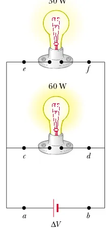
Quick Quiz 27.7
The same potential difference is applied to the twolightbulbs shown in Figure 27.14. Which one of the following statements is true? (a) The 30-W bulb carries the greater current and has the higher resistance. (b) The 30-W bulb carries the greater current, but the 60-W bulb has the higher resistance. (c) The 30-W bulb has the higher resistance, but the 60-W bulb carries the greater current. (d) The 60-W bulb carries the greater current and has the higher resistance.
Quick Quiz 27.8
For the two lightbulbs shown in Figure 27.15, rank thecurrent values at points athrough f, from greatest to least.
Figure 27.14 (Quick Quiz 27.7) These lightbulbs operate at their rated power only when they are connected to a 120-V source.
Figure 27.15 (Quick Quiz 27.8) Two lightbulbs connected across the same potential difference.
George Semple
∆V 30 W
60 W
e f
c d
a b
Example 27.7 Power in an Electric Heater
An electric heater is constructed by applying a potential difference of 120 V to a Nichrome wire that has a total resistance of 8.00'. Find the current carried by the wire and the power rating of the heater.
Solution Because !V"IR, we have
We can find the power rating using the expression ""I2R:
""I 2R"(15.0 A)2(8.00 ')"1.80#103 W
15.0 A I" ∆V
R " 120 V 8.00 ' "
What If? What if the heater were accidentally connected to a 240-V supply? (This is difficult to do because the shape and orientation of the metal contacts in 240-V plugs are different from those in 120-V plugs.) How would this affect the current carried by the heater and the power rating of the heater?
Answer If we doubled the applied potential difference, Equation 27.8 tells us that the current would double. According to Equation 27.23, ""(!V)2/R, the power would be four times larger.
Example 27.8 Linking Electricity and Thermodynamics
Example 27.9 Current in an Electron Beam
(A) What is the required resistance of an immersion heater that will increase the temperature of 1.50 kg of water from 10.0°C to 50.0°C in 10.0 min while operating at 110 V?
(B) Estimate the cost of heating the water.
Solution This example allows us to link our new under-standing of power in electricity with our experience with specific heat in thermodynamics (Chapter 20). An immer-sion heater is a resistor that is inserted into a container of water. As energy is delivered to the immersion heater, raising its temperature, energy leaves the surface of the resistor by heat, going into the water. When the immersion heater reaches a constant temperature, the rate of energy delivered to the resistance by electrical transmission is equal to the rate of energy delivered by heat to the water.
(A) To simplify the analysis, we ignore the initial period during which the temperature of the resistor increases, and also ignore any variation of resistance with temperature. Thus, we imagine a constant rate of energy transfer for the entire 10.0 min. Setting the rate of energy delivered to the resistor equal to the rate of energy entering the water by heat, we have
where Q represents an amount of energy transfer by heat into the water and we have used Equation 27.23 to express
"" (∆V )
2
R " Q ∆t
the electrical power. The amount of energy transfer by heat necessary to raise the temperature of the water is given by Equation 20.4, Q"mc!T. Thus,
Substituting the values given in the statement of the problem, we have
(B) Because the energy transferred equals power multiplied by time interval, the amount of energy transferred is
If the energy is purchased at an estimated price of 10.0¢ per kilowatt-hour, the cost is
0.7 ¢ '
Cost"(0.069 8 kWh)($0.100/kWh)"$0.006 98
"69.8 Wh"0.069 8 kWh "∆t" (∆V)
2
R ∆t"
(110 V)2
28.9 ' (10.0 min)
"
1 h 60.0 min
#
28.9 '"
R" (110 V )
2(600 s)
(1.50 kg)(4186 J/kg( .C)(50.0.C$10.0.C) (∆V )2
R " mc ∆T
∆t 9: R"
(∆V )2 ∆t mc ∆T
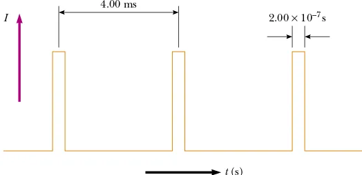
Solution We use Equation 27.2 in the form dQ"I dtand integrate to find the charge per pulse. While the pulse is on, the current is constant; thus,
Dividing this quantity of charge per pulse by the electronic charge gives the number of electrons per pulse:
"5.00#10$8 C
Q pulse"I
$
dt"I ∆t"(250#10$3 A)(200#10$9 s) In a certain particle accelerator, electrons emerge withan energy of 40.0 MeV (1 MeV"1.60#10$13J). The electrons emerge not in a steady stream but rather in pulses at the rate of 250 pulses/s. This corresponds to a time interval between pulses of 4.00 ms (Fig. 27.16). Each pulse has a duration of 200 ns, and the electrons in the pulse constitute a current of 250 mA. The current is zero between pulses.
(A) How many electrons are delivered by the accelerator per pulse?
Interactive
At the Interactive Worked Example link at http://www.pse6.com, you can explore the heating of the water.
I 2.00 × 10⁻⁷s
t (s) 4.00 ms
Summary 849
(B) What is the average current per pulse delivered by the accelerator?
Solution Average current is given by Equation 27.1, Iav " !Q/!t.Because the time interval between pulses is 4.00 ms, and because we know the charge per pulse from part (A), we obtain
This represents only 0.005% of the peak current, which is 250 mA.
(C) What is the peak power delivered by the electron beam? Solution By definition, power is energy delivered per unit time interval. Thus, the peak power is equal to the energy delivered by a pulse divided by the pulse duration:
10.0 MW
"1.00#107 W"
#
"
1.60#10$13 J
1 MeV
#
" (3.13#10
11 electrons/pulse)(40.0 MeV/electron)
2.00#10$7 s/pulse (1)
"peak" pulse energy
pulse duration 12.5 /A Iav"
Q pulse ∆t "
5.00#10$8 C 4.00#10$3 s "
3.13#1011 electrons/pulse
"
Electrons per pulse" 5.00#10
$8 C/pulse
1.60#10$19 C/electron
We could also compute this power directly. We assume that each electron has zero energy before being accelerated. Thus, by definition, each electron must go through a potential difference of 40.0 MV to acquire a final energy of 40.0 MeV. Hence, we have
What If? What if the requested quantity in part (C) were the
averagepower rather than the peakpower?
Answer Instead of Equation (1), we would use the time interval between pulses rather than the duration of a pulse:
Instead of Equation (2), we would use the average current found in part (B):
Notice that these two calculations agree with each other and that the average power is much lower than the peak power.
"500 W
"av"Iav ∆V"(12.5#10$6 A)(40.0#106 V)
"500 W
#
"
1.60#10$13 J
1 MeV
#
" (3.13#10
11 electrons/pulse)(40.0 MeV/electron)
4.00#10$3 s/pulse
"av" pulse energy time interval between pulses
10.0 MW
"
"(250#10$3 A)(40.0#106 V) (2)
"peak"Ipeak ∆V
The electric currentIin a conductor is defined as
(27.2)
where dQis the charge that passes through a cross section of the conductor in a time interval dt. The SI unit of current is the ampere(A), where 1 A"1 C/s.
The average current in a conductor is related to the motion of the charge carriers through the relationship
(27.4)
where nis the density of charge carriers, qis the charge on each carrier, vdis the drift speed, and Ais the cross-sectional area of the conductor.
The magnitude of the current density J in a conductor is the current per unit area:
(27.5) J ! I
A "nqvd Iav"nqvdA
I ! dQ dt
S U M M A R Y
Take a practice test for this chapter by clicking on the Practice Test link at
The current density in an ohmic conductor is proportional to the electric field according to the expression
(27.7)
The proportionality constant &is called the conductivityof the material of which the conductor is made. The inverse of & is known as resistivity % (that is, % "1/&). Equation 27.7 is known as Ohm’s law,and a material is said to obey this law if the ratio of its current density Jto its applied electric field Eis a constant that is independent of the applied field.
The resistanceRof a conductor is defined as
(27.8)
where !Vis the potential difference across it, and Iis the current it carries.
The SI unit of resistance is volts per ampere, which is defined to be 1 ohm ('); that is, 1' "1 V/A. If the resistance is independent of the applied potential difference, the conductor obeys Ohm’s law.
For a uniform block of material of cross sectional area A and length !, the resistance over the length !is
(27.11)
where %is the resistivity of the material.
In a classical model of electrical conduction in metals, the electrons are treated as molecules of a gas. In the absence of an electric field, the average velocity of the electrons is zero. When an electric field is applied, the electrons move (on the average) with a drift velocity vdthat is opposite the electric field and given by the expression
(27.14)
where +is the average time interval between electron–atom collisions, meis the mass of the electron, and q is its charge. According to this model, the resistivity of the metal is
(27.17)
where nis the number of free electrons per unit volume.
The resistivity of a conductor varies approximately linearly with temperature according to the expression
(27.19)
where -is the temperature coefficient of resistivityand %0is the resistivity at some reference temperature T0.
If a potential difference !Vis maintained across a circuit element, the power,or rate at which energy is supplied to the element, is
(27.22)
Because the potential difference across a resistor is given by !V"IR, we can express the power delivered to a resistor in the form
(27.23)
The energy delivered to a resistor by electrical transmission appears in the form of internal energy in the resistor.
""I2R" (∆V )
2
R ""I!V % " %0[1,-(T$T0)]
% " me nq2+
vd"
qE
me + R"% !
A
R ! ∆V
I