A. Data presentation - The Effect Of Using Total Physical Response (Tpr) Method On Vocabulary Size At Seventh Grade Students Of MTs Muslimat NU Palangkaraya - Digital Library IAIN Palangka Raya

(1)

CAPTER IV

RESEARCH FINDINGS AND DISCUSSIONS

In this chapter, the writer discussed the result of the study which covered the data presentation, the result of data analysis, and discussion.

A. Data presentation

This section consists of the measurement of central tendency (mean, median, and mode of each group score), the measurement of variability (standard deviation and standard error of the mean), some figures and tables of each group score and the discussion of the study.

1. The Result of Pretest Experimental Group and Control Group a. Distribution of Pretest Scores of the Experimental Group

The test scores of experimental group were presented in the following table: Table 4.1

The Description of Pre test. Scores of the Data Achieved By the Students in Experimental Group

Student’s Code Score

E01 34

E02 40

E03 35

E04 45

E05 40

E06 50

(2)

E08 50

E09 30

E10 40

E11 55

E12 59

E13 50

E14 37

E15 36

E16 45

E17 35

E18 35

E19 40

E20 56

E21 36

E22 55

E23 37

E24 36

E25 40

E26 45

E27 50

E28 30

E29 38

E30 40

E31 40

E32 35

(3)

E34 55

E35 40

Based on the data above, it can be seen that the students’ highest score was

59 and the student’s lowest score was 30. To determine the range of score, the class interval, and interval of temporary, the writer calculated using formula as follows:

The Highest Score (H) = 59 The lowest Score (L) = 30 The Range of Score (R) = H-L+1

= 59 – 30 + 1 = 29 + 1 = 30 The Class Interval (K) =1+ (3.3) x Log n

= 1+ (3.3) x Log 35

= 1+ (3.3) x 1, 5440680444 = 6, 0954245464 = 6

Interval of Temporary =

K R

= = 5

(4)

Table 4.2

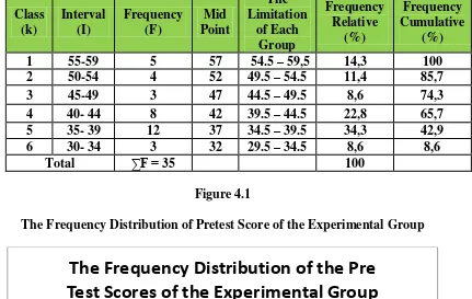
The Frequency Distribution of the Pre test. Score of the Experimental Group

Class

The Frequency Distribution of Pretest Score of the Experimental Group

It can be seen from the figure above, the students’ pretest scores in

experimental group. There were three student who got score 29,5-34,5. There were twelve students who got score 34,5-39,5. There were eight students who got score 39,5-44,5. There were three students who got score 44,5-49,5. There were

y The Limitation of Each Group

(5)

four students who got score 49,5-54,5. And there was five students who got score 54,5-59,5.

The next step, the writer tabulated the scores into the table for the calculation of mean, median, and modus as follows:

Table 4.3

The Calculating Mean, Median, and modus of Pretest Score of the Experimental Group

Interval (I) Frequency (F)

Mid Point

(X)

FX Fkb Fka

55-59 5 57 285 35 3

50-54 4 52 208 30 8

45-49 3 47 141 26 12

40- 44 8 42 336 23 15

35- 39 12 37 444 15 23

30- 34 3 32 96 3 35

∑F = 35 ∑Fx =1510

a) Mean

Mx = N fX



=

= 43,1 b)Median

Mdn =

(6)

= 39, 5+ 1,6 = 41,1 c) Modus

Mo = + ( )

= 39, 5+

= 39, 5 +

_{= 39, 5 + 0} = 39,5

The calculation above showed of mean value was 43,1, median value was 47,2 and modus value was 39,5 of the pre test of the experiment group. The last step, the writer tabulated the scores of pre test of experiment group into the table for the calculation of standard deviation and the standard error as follows:

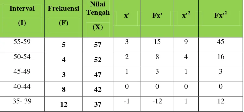
Table 4.4

The Calculation of the Standard Deviation and the Standard Error of the Pre Test Scores of experiment Group

Interval (I)

Frekuensi (F)

Nilai Tengah

(X)

x' Fx' x'2 Fx'2

55-59 ₅ ₅₇ 3 15 9 45

50-54 ₄ ₅₂ 2 8 4 16

45-49 ₃ ₄₇ 1 3 1 3

40-44 ₈ ₄₂ 0 0 0 0

(7)

30-34 ₃ ₃₂ -2 -6 4 12

Total N=35 ∑Fx’= 8 ∑Fx’2= 88

a) Standard Deviationn

 

b)Standard Error

(8)

The result of calculation showed the standard deviation of pre test score of experiment was 7,81 and the standard error of pre test score of experiment group was 1,34.

The writer also calculated the data calculation of post test score of experimental group using SPSS 16 program. The result of statistic table is as follows:

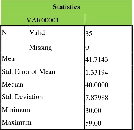
Table 4.5

The Table of Calculation of Mean, Standard Deviation, and Standard Error of Mean of Pre-Test Score in Experimental Group Using SPSS 16 Programs

Statistics VAR00001

N Valid ₃₅

Missing 0

Mean 41.7143

Std. Error of Mean 1.33194

Median 40.0000

Std. Deviation 7.87988

Minimum 30.00

(9)

The table showed the result of mean calculation was 41.7143. The result of standard deviation was 7.87988 and the result of standard error of mean calculation was 1.33194.

b. Distribution of Pre Test Scores of the Control Group

The pre test scores of the control group were presented in the following table:

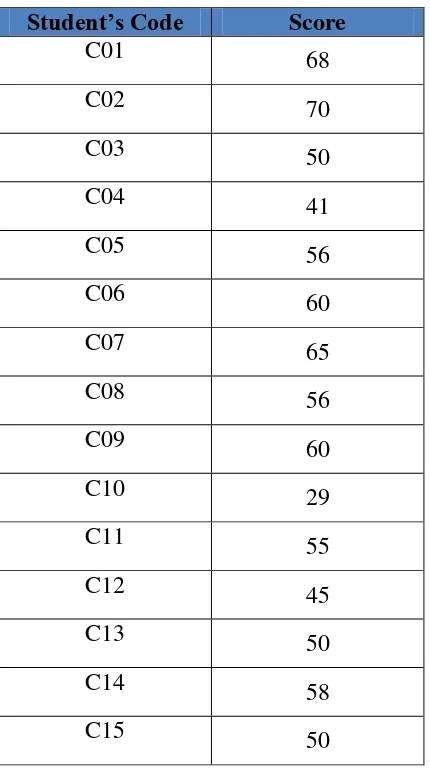
Table 4.6

The Description of Pretest Scores of the Data Achieved by the Students in Control Group

C01 ₆₈

C02 ₇₀

C03 ₅₀

C04 ₄₁

C05 ₅₆

C06 ₆₀

C07 ₆₅

C08 ₅₆

C09 ₆₀

C10 ₂₉

C11 ₅₅

C12 ₄₅

C13 ₅₀

C14 ₅₈

(10)

C16 ₅₄

C17 ₇₀

C18 ₅₈

C19 ₄₈

C20 ₅₃

C21 ₅₉

C22 ₅₈

C23 ₅₀

C24 ₅₇

C25 ₅₃

C26 ₅₉

C27 ₅₆

C28 ₇₀

C29 ₆₄

C30 ₅₂

C31 ₆₈

C32 ₇₀

C33 36

C34 55

C35 40

(11)

The Highest Score (H) = 70

The Frequency Distribution of the Pretest Scores of the Control Group

(12)

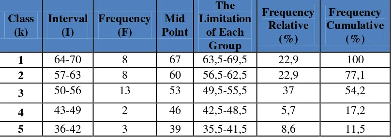
6 29-35 1 32 28,5-34,5 2,9 2,9

Total ∑F 35 ∑P = 100

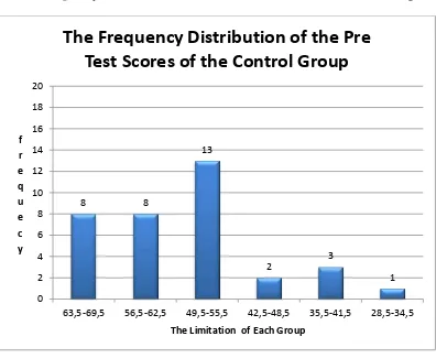
Figure 4.2

The Frequency Distribution of the Pre test Scores of the Control Group

It can be seen from the figure above, the students’ pretest scores in control group. There were one students who got score 28,5-34,5. There were three students who got score 35,5-41,5. There were two students who got score 42,2-48,5. There were thirteen students who got score 49,5-55,5. There were eight students who got score 56,5-62,5.And there was eight student who got score 63,5-69,5.

The next step, the writer tabulated the scores into the table for the calculation of mean, median, and modus as follows:

8 8

13

2

3

1

0 2 4 6 8 10 12 14 16 18 20

63,5-69,5 56,5-62,5 49,5-55,5 42,5-48,5 35,5-41,5 28,5-34,5 f

r e

q u e

c y

The Limitation of Each Group

(13)

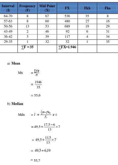
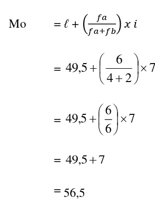
Table 4.8

(14)

c) Modus 55,7 and modus value was 56,5 of the pre test of the control group.

The last step, the writer tabulated the scores of pre test of control group into the table for the calculation of standard deviation and the standard error as follows:

Table 4.9

The Calculation of the Standard Deviation and the Standard Error of the Pre Test Scores of Control Group

(15)

Total N=35 ∑Fx’= 48

∑Fx’2 =124

a) Standard Deviation

 

1

(16)

Table 4.10

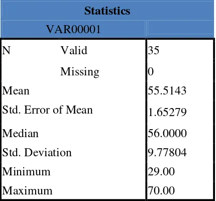
The Table of Calculation of Mean, Standard Deviation, and Standard Error of Mean of Pre-Test Score in Control Group Using SPSS 16 Programs

N Valid 35

Missing 0

Mean 55.5143

Std. Error of Mean _1.65279

Median 56.0000

Minimum 29.00

Maximum 70.00

The table showed the result of mean calculation was 55,5. The result of standard deviation was 9,77 and the result of standard error of mean calculation was 1,652.

2. The Result of Post-test Experimental Group and Control Group a. Distribution of Post Test Scores of the Experimental Group

(17)

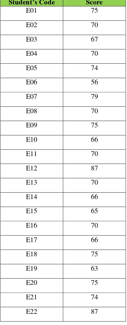
Table 4.11

The Description of Post Test Scores of the Data Achieved by the Students in Experimental Group

E01 75

E02 70

E03 67

E04 70

E05 74

E06 56

E07 79

E08 70

E09 75

E10 66

E11 70

E12 87

E13 70

E14 66

E15 65

E16 70

E17 66

E18 75

E19 63

E20 75

E21 74

(18)

E23 87

E24 62

E25 87

E26 66

E27 87

E28 66

E29 74

E30 62

E31 74

E32 70

E33 58

E34 58

E35 60

The Highest Score (H) = 87 The Lowest Score (L) = 58

The Range of Score (R) = H – L + 1 = 87 – 58 + 1 = 30

The Class Interval (K) = 1 + (3.3) x Log n = 1 + (3.3) x Log 35 = 1 + (3.3) x 1,544 = 1 + 1,544

(19)

Interval of Temporary (I) =

6 30 

K R

= ₅

So, the range of score was 30, the class interval was 6, and interval of temporary was 5. It was presented using frequency distribution in the following table:

Table 4.12

Frequency Distribution of the Pos-Test Score of the Experimental Group

Class (k)

Frequency (F)

Mid Point

The Limitation

of Each Group

Frequency Relative

(%)

Frequency Cumulative

(%)

1 83-87 5 85 82,5-86,5 14,29 100

2 78-82 1 80 77,5-81,5 2,85 85,71

3 73-77 8 75 72,5-76,5 22,86 82,86

4 68- 72 8 70 67,5-71,5 22,86 60

5 63- 67 8 65 62,5-66,5 22,86 37,14

6 58- 62 5 60 57,5-61,5 14,28 14,28

(20)

Figure 4.3

The Frequency Distribution of Pos-test Score of the Experimental Group

experimental group. There were five students who got score 82,5-86,5. There was one student who got score 77,5-81,5. There were eight students who got score 72,5-76,5. There were eight students who got score 67,5-71,5. There were eight students who got score 62,5- 66,5. And there was five student who got score 57,5- 61,5.

The next step, the writer tabulated the scores into the table for the calculation of mean, median, and modus as follows.

5

1

8 8 8

5

0 2 4 6 8 10 12

82,5-86,5 77,5-81,5 72,5-76,5 67,5-71,5 62,5-66,5 57,5-61,5 f

r e q u

e c y

(21)

Table 4.13

The Calculating Mean, Median, and Modus of Post-test Score of the Experimental Group

Mid Point

(X) FX Fkb Fka

83-87 5 85 425 35 5

78-82 1 80 80 30 6

73-77 8 75 600 29 14

68- 72 8 70 560 21 22

63- 67 8 65 520 13 30

58- 62 5 60 300 5 35

∑F = 35 ∑Fx =

2485 a) Mean

Mx = N

fX



=

= 71 b)Median

Mdn =

= = 67,5 + 2,81 = 70,31 c) Modus

(22)

= 67,5+

= 67,5 +

= 67,5 + 3,1 = 71

The calculation above showed of mean value was 71, median value was 75,31 and modus value was 75,6 of the Pos test of the Experiment group.

The last step, the writer tabulated the scores of pre test of experiment group into the table for the calculation of standard deviation and the standard error as follows:

Table 4.14

The Calculation of the Standard Deviation and the Standard Error of the Post Test Scores of experiment Group

Mid Point

(X) x' Fx' x'

2

Fx'2

83-87 5 85 3 15 10 50

78-82 1 80 2 2 4 4

73-77 8 75 1 8 2 64

68- 72 8 70 0 0 0 0

63- 67 8 65 -1 -8 1 64

58- 62 5 60 -2 -10 4 9

∑F = 35 ∑Fx’=

43

(23)

1

(24)

Table 4.15

The Table of Calculation of Mean, Standard Deviation, and Standard Error of Mean of Post-Test Score in Experimental Group Using SPSS 16 Programs

N Valid 35

Missing 0

Mean 70.8857

Median 70.0000

Range 31.00

Minimum 56.00

Maximum 87.00

b. Distribution of Post Test Scores of the Control Group

(25)

Table 4.16

The Description of Post Test Scores of the Data Achieved by the Students in Control Group

C01 ₇₀

C02 ₇₀

C03 ₇₀

C04 ₆₅

C05 ₆₇

C06 ₆₀

C07 ₆₅

C08 ₆₀

C09 ₆₀

C10 ₄₁

C11 ₇₀

C12 ₄₅

C13 ₆₇

C14 ₅₈

C15 ₆₀

C16 ₅₄

C17 ₇₀

C18 ₅₈

C19 ₄₈

C20 ₅₃

C21 ₅₉

(26)

C23 ₇₀

C24 ₅₇

C25 ₅₃

C26 ₇₀

C27 ₅₆

C28 ₇₀

C29 ₆₄

C30 ₅₂

C31 ₆₈

C32 ₇₀

C33 41

C34 55

C35 41

70 and the student’s lowest score was 41. To determine the range of score, the class interval, and interval of temporary, the writer calculated using formula as follows:

The Highest Score (H) = 70 The Lowest Score (L) = 41

The Range of Score (R) = H – L + 1 = 70 –41 + 1 = 30

(27)

= 1 + (3.3) x 1,5440680444 = 6,095

= 6 Interval of Temporary (I) =

6 30 

K R

= ₅

So, the range of score was 30, the class interval was 6, and interval of temporary was 5. Then, it was presented using frequency distribution in the following table:

Table 4.17

Frequency Distribution of the Pos-Test Score of the Control Group

Class (k)

Frequency

(F) Mid Point

The Limitation

of Each Group

Frequency Relative

(%)

Frequency Cumulative

(%)

1 66-70 12 68 65,5-69,5 34,28 100

2 61-65 3 63 60,5-64,5 8,56 65,72

3 56-60 10 58 55,5-59,5 28,55 57,16

4 51-55 5 53 50,5-54,5 14,28 28,61

5 46-50 1 48 45,5-49,5 2,9 14,33

6 41-45 4 43 40,5-44,5 11,43 11,43

(28)

Figure 4.4

The Frequency Distribution of the Post Test Scores of the Control Group

experimental group. There were twolevee students who got score 65,5-69,5. There were three students who got score 60,5-64,5. There were teen students who got score 55,5-59,5. There were five students who got score 50,5-54,5. There were one students who got score 45,5-49,5.And there was four student who got score 40,5-44,5.

Table 4.18

The Calculating Mean of Post-test Score of the Control Group

(29)

(30)

The calculation above showed of mean value was 59 , median value was 59 , and modus value was 62 of the pos test of the control group.

The last step, the writer tabulated the scores of pos test of control group into the table for the calculation of standard deviation and the standard error as follows:

Table 4.19

The Calculation of the Standard Deviation and the Standard Error of the Post Test Scores of control Group

(31)

038

b) Standard Error

1

The result of calculation showed the standard deviation of post-test score of control group was 10 and the standard error of pos test score of control group was 1,7.

(32)

Table 4.20

The Table of Calculation of Mean, Standard Deviation, and Standard Error of control Group Using SPSS 16 Program

N Valid 35

Missing 0

Mean 59.8571

Median 60.0000

Range 29.00

Minimum 41.00

Maximum 70.00

3. Testing the Normality and the Homogeneity

(33)

the distribution is normal.1 Then, the homogeneity is used to know the data were homogeny or not.

a. The Normality of Post Test Score in Experiment and Control Group Table 4.21

The Test Normality of Posttest Score

GROUP

Kolmogorov-Smirnova Shapiro-Wilk Statistic df Sig. Statistic df Sig.

SCORE X1 .146 35 .058 .930 35 .028

X2 .134 35 .117 .897 35 .013

From the table of Kolmogorov-Swirnov, the writer concluded that the significance of experiment group was 0.028 and the significance of control group was 0,003. It was higher than the signifcance 0,058. Thus, the distribution of the data was said to be in normal distribution.

1

(34)

b. Testing of Homogeneity of Posttest Score of Experiment and Control Group.

Table 4.22

Test of Homogeneity

Test of Homogeneity of Variance Levene

Statistic df1 df2 Sig.

SCORE Based on Mean .252 1 68 .617

Based on Median .377 1 68 .541

Based on Median and

with adjusted df .377 1 67.789 .541

Based on trimmed mean .302 1 68 .585

Based on the table above, the result of the analysis using SPSS program showed that the Levene Statistic was 252, the df1 was 1 and df2 was 68 and the value of signifance (sig.) was 0.617. The writer concluded that the homogeneity of posttest score of experimental and control group was accepted because the value of significance (sig. 0,617) was higher that significance level (sig. 0,05). Thus, it was said that the data were homogeneous.

B. Result of Data Analysis

1. Testing Hypothesis Using Manual Calculation

(35)

level at 5% due to the Hypothesis type stated on non-directional (two-tailed test). It meant that the Hypothesis cannot direct the prediction of alternative Hypothesis. To test the hypothesis of the study, the writer used t-test statistical calculation. Firstly, the writer calculated the standard deviation and the error of X1 and X2. It was found the Standard deviation and the Standard error of post test of X1 and X2 at the previous data presentation. It could be seen on this following table:

Table 4.23

The Standard Deviation and Standard Error of X1 and X2

Variable The Standard Deviation The Standard Error

X1 9,9 1,6

X2 10 1,7

Where:

X1 : Experimental Group X2 : Control Group

The table showed the result of the standard deviation calculation of X1 was 9,9 and the result of the standard error mean calculation was 1,6. The result of the standard deviation calculation of X2 was 10 and the result of the standard error mean calculation was 1.7.

The next step, the writer calculated the standard error of the differences mean between X1 and X2 as follows:

(36)

SEM1 – SEM2 =

2 2

2

1 SEm

SEm 

SEM1 – SEM2 = 1,342 1.772 SEM1 – SEM2 = 1,79563,1329 SEM1 – SEM2 = 4,9285

SEM1 – SEM2 = 2,22 SEM1 – SEM2 = 2,22

The calculation above showed the standard error of the differences mean between X1 and X2 was 2,22. Then, it was inserted to the to formula to get the value of t observe as follows:

to =

2 1

SEm SEm

M M

 

to =

2,22 59 71

to =

2,22 12

to = 5,405 With the criteria:

If t-test (t-observed) ≥ t-table, Ha is accepted and Ho is rejected. If t-test (t-observed) < t-table, Ha is rejected and Ho is accepted.

Then, the writer interpreted the result of t-test. Previously, the writer accounted the degree of freedom (df) with the formula:

(37)

ttable at df 68 at 5% significant level = 2.650

The writer chose the significant levels on 5%; it means the significant level of refusal of null hypothesis on 5%. The writer decided the significance level at 5% due to the hypothesis typed stated on non-directional (two-tailed test). It

meant that the hypothesis can’t direct the prediction of alternative hypothesis. The calculation above showed the result of t-test calculation as in the table follows:

Table 4.24 The Result of T-test

Variable T observed T table Df/db

5% 1%

X1-X2 5,405 2.650 3,214 68

Where:

X1 = Experimental Group X2 = Control Group

T observe = The Calculated Value T table = The Distribution of t value Df/db = Degree of Freedom

Based on the result of hypothesis test calculation, it was found that the value of tobserved was greater than the value of ttable at significance level or 2.650 < 5,405 > 3,214. It meant Ha was accepted and Ho was rejected.

(38)

those taught using Direct Method was accepted and Ho stating that the students taught by Total Physical Response do not have better vocabulary size than those taught using Direct Method was rejected. Therefore teaching using Total Physical Response gave significant effect on the student’s vocabulary size of the student’s seventh grade of MTs Muslimat NU Palangka Raya.

2. Testing Hypothesis Using SPPS Program

The writer also applied SPSS 16 program to calculate t test in testing hypothesis of the study. The result of t test using SPSS 16 was used to support the manual calculation of the t test. The result of the t test using SPSS 16 program could be seen as follows:

Table 4.25

The Standard Deviation and the Standard Error of X1 and X2

Group N Mean Std. Deviation Std. Error Mean

Score X1 35 70,8857 8,63907 1,46027

X2 35 59,8571 9,13990 1,54493

(39)

Table 4.26

The Calculation T-test Using SPPS 16 program Independent Samples Test

Independent Samples Test Levene's

Test for Equality of

Variances

t-test for Equality of Means

F Sig. t df Sig.

(2-tailed

)

Mean Differenc

e

Std. Error Difference

95% Confidence Interval of the

Difference Lower Upper

Score

Equal variances

assumed

,252 ,617 5,405 68 0,541 11,02857 2,12584 6,78653 15,27061 Equal

variances not assumed

5,405 67,785 0,541 11,02857 2,12584 6,78629 15,27086

Based on the result of t-value using SPSS 16 program. Since the result of post test between experimental and control group had difference score of variance, it found that the result of t observed was 5,405, the result of mean difference between experimental and control group was 11,02857.

(40)

freedom (df) was 68. The following table was the result of t observed and t table

from 68 df at 5% and 1 % significance level.

Table 4.27

The Result of T-test

Variable t observe t table Df/db

5% 1%

X1- X2 5,405 2.650 3,214 68

Where:

X1 = Experimental Group

X2 = Control Group

T observe = the Calculated Value T table = The Distribution of t value Df/db = Degree of Freedom

C. Discussion

The result of the analysis shows that Total Physical Response gives significant effect to the students’ vocabulary size. It could be proved from the

(41)

To support the result of testing hypothesis, the writer also calculated the hypothesis using SPSS 16 program. The result of the analysis showed that the students who are taught by using Total Physical Response method gave significant

effect on the students’ _{vocabulary size. It is proved by the value of t}observeb_that

was higher than ttable_{, either at 5% significance level or at 1% significance level} (2,650 <5,405 < 2,314).

Those statistical findings were suitable with the theories as mentioned before. Total Physical Response method do promote language learning for they not only aid pronunciation, make vocabulary and structures memorable but also bring variety and fun to the language learning classroom

A method or technique in teaching and learning process must be developed in order to get a better purpose for a better life. TPR was developed in order to improve the better result of teaching learning process of a new language. Teachers who use TPR believe in the importance of having the students enjoy their experience in learning to communicate a foreign language.

According to Larsen-Freeman, TPR was develop in order to reduce the stress people feel when studying foreign language and thereby encourage students to persist in their study beyond a beginning level of proficiency.2

These findings were suitable with the theories as stated in chapter II. The first, Total Physical Response method was an interesting technique for the students because itwas a completely technique for the students at MTs Muslimat

2

(42)

NU Palangka Raya It was shows from the students’ response that they were very enjoy in classroom.

Second, vocabulary size was the important one in learning English. It was the obligation of this school. It could help the students to vocabulary size. It also

made the students aware of materials that were not essential to the students’

memorizing to be deleted. So, Total Physical response method are suitable for all students no matter what age they are and what level of English, learning strategies, intelligence, interests or learning problems they have.

There are reasons why Total Physical Response gives effect on the students’ vocabulary seventh grade students at MTs Muslimat NU Palangka Raya. First, using Total Physical Response, the students could easy and fun to memories words or vocabulary. Students get greatly motivated by using word in the foreign language classroom. TPR Method creates an atmosphere of interest in the study of

English and can lead from a “teacher centered” to a “student centered” class”. So,

Students become themselves when they want to speak in the class.

And the lastone problem, which TPR method has related its special reliance on action (Physical Response). For social reason, many adults and children, feel

embarrassed marching around a room to do the teacher’s comments. For that, the

(43)

Based on the evidence above, it could be concluded that the idea

development quality of students’ vocabulary size was better by using total