A Modeling Framework for Simulating River and Stream Water Quality

A Modeling Framework for Simulating River and Stream Water Quality

Documentation and

Users Manual

The Mystic River at Medford, MA

Steve Chapra and Greg Pelletier

November 25, 2003

1 INTRODUCTION

QUAL2K (or Q2K) is a river and stream water quality model that is intended to represent a modernized version of the QUAL2E (or Q2E) model (Brown and Barnwell 1987). Q2K is similar to Q2E in the following respects:

• One dimensional. The channel is well-mixed vertically and laterally. • Steady state hydraulics. Non-uniform, steady flow is simulated.

• Diurnal heat budget. The heat budget and temperature are simulated as a function of meteorology on a diurnal time scale.

• Diurnal water-quality kinetics. All water quality variables are simulated on a diurnal time scale.

• Heat and mass inputs. Point and non-point loads and abstractions are simulated.

The QUAL2K framework includes the following new elements:

• Software Environment and Interface. Q2K is implemented within the Microsoft Windows environment. It is programmed in the Windows macro language: Visual Basic for

Applications (VBA). Excel is used as the graphical user interface.

• Model segmentation. Q2E segments the system into river reaches comprised of equally spaced elements. In contrast, Q2K uses unequally-spaced reaches. In addition, multiple loadings and abstractions can be input to any reach.

• Carbonaceous BOD speciation. Q2K uses two forms of carbonaceous BOD to represent organic carbon. These forms are a slowly oxidizing form (slow CBOD) and a rapidly oxidizing form (fast CBOD). In addition, non-living particulate organic matter (detritus) is simulated. This detrital material is composed of particulate carbon, nitrogen and phosphorus in a fixed stoichiometry.

• Anoxia. Q2K accommodates anoxia by reducing oxidation reactions to zero at low oxygen levels. In addition, denitrification is modeled as a first-order reaction that becomes pronounced at low oxygen concentrations.

• Sediment-water interactions. Sediment-water fluxes of dissolved oxygen and nutrients are simulated internally rather than being prescribed. That is, oxygen (SOD) and nutrient fluxes are simulated as a function of settling particulate organic matter, reactions within the sediments, and the concentrations of soluble forms in the overlying waters.

• Bottom algae. The model explicitly simulates attached bottom algae.

• Light extinction. Light extinction is calculated as a function of algae, detritus and inorganic solids.

• pH. Both alkalinity and total inorganic carbon are simulated. The river’s pH is then simulated based on these two quantities.

2 GETTING

STARTED

Installation is required for many water-quality models. This is not the case for QUAL2K because the model is packaged as an Excel Workbook. The program is written in Excel’s macro language: Visual Basic for Applications or VBA. The Excel Workbook’s worksheets and charts are used to enter data and display results. Consequently, you merely have to open the Workbook to begin modeling. The following are some recommended step-by-step instructions on how to obtain your first model run.

Step 1: Create a folder named QUAL2K to hold the workbook and its data files. For example, in the following example, a folder named QUAL2K is created on the C:\ drive.

Step 2: Copy the Q2KMaster file (Q2KMaster.xls) from your CD to C:\QUAL2K.

Step 3: Open Excel and make sure that your macro security level is set to medium (Figure 1). This can be done using the menu commands: Tools → Macro → Security. Make certain that the Medium radio button is selected.

Figure 1 The Excel Macro Security Level dialogue box. In order to run Q2K, the Medium level of security should be selected.

Figure 2 The Excel Macro security dialogue box. In order to run Q2K, the Enable Macros button must be selected.

Click on the Enable Macros button.

Step 5: Immediately save the file as Q2K.xls. This will be the Excel Workbook that you will use on a routine basis. If for some reason, you modify Q2K.xls in a way that makes it unusable, you can always go back to Q2KMaster.xls as a backup.

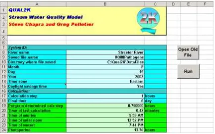
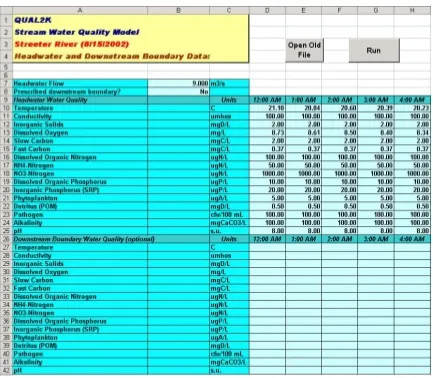
Step 6: On the QUAL2K worksheet, go to cell B10 and enter the path to the DataFiles directory: C:\QUAL2K\DataFiles as shown in Figure 3.

Figure 3 The QUAL2K worksheet showing the entry of the file path into cell B10.

Figure 4 The QUAL2K Status Bar is positioned at the lower left corner of the worksheet. It allows you to follow the progress of a model run.

If the program runs properly, the temperature plot will be displayed. If it does not work properly, two possibilities exist:

First, you may be using an old version of Microsoft Office. Although Excel is downwardly compatible for some earlier versions, Q2K will not work with very old versions.

Second, you may have made a mistake in implementing the preceding steps. A common mistake is to have mistyped the file path that you entered in cell B10. If this is the case, you will receive an error message (Figure 5).

Figure 5 An error message that will occur if you type the incorrect file path into cell B10 on the QUAL2K worksheet.

If this occurs, click on the end button. This will terminate the run and bring you back to the Excel Workbook. You should then move back to the QUAL2K worksheet and correct the file path entry. Note that the same error will occur if you did not set up your directories with correct names as specified above.

Step 8: On the QUAL2K worksheet click on the Open Old File button. Browse to get to the directory: C:\QUAL2K\DataFiles. You should see that a new file: BC092187.q2k has been created. Click on the Cancel button to return to Q2K.

3 SEGMENTATION

AND

HYDRAULICS

The model presently simulates the main stem of a river as depicted in Figure 6. Tributaries are not modeled explicitly, but can be represented as point sources.

1

2

3

4 5 6

8 7

Non-point abstraction

Non-point source Point source

Point source Point abstraction

Point abstraction Headwater boundary

Downstream boundary Point source

Figure 6 QUAL2K segmentation scheme.

3.1 Flow Balance

A steady-state flow balance is implemented for each model reach (Figure 7)

i ab i in i

i Q Q Q

Q = ₋₁+ _, − _, (1)

where Qi = outflow from reach i into reach i + 1 [m3/d], Qi–1 = inflow from the upstream reach i –

1 [m3/d], Qin,i is the total inflow into the reach from point and nonpoint sources [m

3

/d], and Qab,i is

the total outflow from the reach due to point and nonpoint abstractions [m3/d].

i

i

+ 1

i

−−−−

1

Q

_{i−−−−1}

Q

_i

Q

_in,i

Q

_ab,i

The total inflow from sources is computed as of non-point source inflows to reach i.

The total outflow from abstractions is computed as

∑

and npai = the total number of non-point abstraction flows from reach i.

The point sources and abstractions are modeled as line sources. As in Figure 8, the non-point source or abstraction is demarcated by its starting and ending kilometer non-points. Its flow is distributed to or from each reach in a length-weighted fashion.

Q_npt

25%Q_npt 25%Q_npt 50%Q_npt

start end

Figure 8 The manner in which non-point source flow is distributed to a reach.

3.2 Hydraulic Characteristics

Once the outflow for each reach is computed, the depth and velocity are calculated in one of three ways: weirs, rating curves, and Manning equations. The program decides among these options in the following manner:

• If the weir height is zero and a roughness coefficient is entered (n), the Manning equation option is implemented.

• If neither of the previous conditions are met, Q2K uses rating curves.

3.2.1 Weirs

Figure 9 shows how weirs are represented in Q2K. The symbols are defined as: Hi = the depth of

the reach upstream of the weir [m], Hi+1 = the depth of the reach downstream of the weir [m],

elev2i = the elevation above sea level of the upstream reach [m], elev1i+1 = the elevation above sea

level of the downstream reach [m], Hw = the height of the weir above elev2i [m], Hd = the drop

Figure 9 A sharp-crested weir.

For a sharp-crested weir where Hh/Hw < 0.4, flow is related to head by (Finnemore and

Franzini 2002)

2

where Qi is the outflow from the segment upstream of the weir in m

3

This result can then be used to compute the depth of reach i, and the drop over the weir

h

i i i

c B H

A_, = (8)

i c

i i

A Q U

,

= (9)

3.2.2 Rating

Curves

Power equations can be used to relate mean velocity and depth to flow,

b

aQ

U

=

(10)

β

α

Q

H

=

(11)

where a, b, α and β are empirical coefficients that are determined from velocity-discharge and stage-discharge rating curves, respectively. The values of velocity and depth can then be employed to determine the cross-sectional area and width by

U Q

A_c = (12)

H A

B= c (13)

The exponents b and β typically take on values listed in Table 1. Note that the sum of b and β must be less than or equal to 1. If their sum equals 1, the channel is rectangular.

Table 1 Typical values for the exponents of rating curves used to determine velocity and depth from flow (Barnwell et al. 1989).

Equation Exponent Typical value Range

b aQ

U = b 0.43 0.4−0.6

H=αQβ β 0.45 0.3−0.5

3.2.3 Manning

Equation

Each reach is idealized as a trapezoidal channel (Figure 10). Under conditions of steady flow, the Manning equation can be used to express the relationship between flow and depth as

3 / 2

3 / 5 2 / 1 0

P

A

n

S

where Q = flow [m3/s]1, S0 = bottom slope [m/m], n = the Manning roughness coefficient, Ac =

Figure 10 Trapezoidal channel. The cross-sectional area of a trapezoidal channel is computed as

[

B s s H

]

H

A_c = ₀+0.5( _s1+ _s2) (15)

where B0 = bottom width [m], ss1 and ss2 = the two side slopes as shown in Figure 10 [m/m], and

H = reach depth [m].

The wetted perimeter is computed as

1

After substituting Equations (15) and (16), Equation (14) can be solved iteratively for depth (Chapra and Canale 2002),

[

B s s H

]

estimated error falls below a specified value of 0.001%. The estimated error is calculated as

%

The cross-sectional area can be determined with Equation (15) and the velocity can then be determined from the continuity equation,

1

c A

Q

U = (19)

The average reach width, B [m], can be computed as

H A

B= c (20)

Suggested values for the Manning coefficient are listed in Table 2.

Table 2 The Manning roughness coefficient for various open channel surfaces (from Chow et al. 1988).

MATERIAL n

Man-made channels

Concrete 0.012 Gravel bottom with sides:

concrete 0.020

mortared stone 0.023

riprap 0.033

Natural stream channels

Clean, straight 0.025-0.04

Clean, winding and some weeds 0.03-0.05 Weeds and pools, winding 0.05 Mountain streams with boulders 0.04-0.10 Heavy brush, timber 0.05-0.20

Manning’s n typically varies with flow and depth (Gordon et al, 1992). As the depth

decreases at low flow, the relative roughness increases. Typical published values of Manning’s n, which range from about 0.015 for smooth channels to about 0.15 for rough natural channels, are representative of conditions when the flow is at the bankfull capacity (Rosgen, 1996). Critical conditions of depth for evaluating water quality are generally much less than bankfull depth, and the relative roughness may be much higher.

3.2.4 Waterfalls

H

_i+1

H

_i

H

_d

elev

2

_i

elev

1

_i+1

Figure 11 Waterfall.

QUAL2K computes such drops for cases where the elevation above sea level drops abruptly at the boundary between two reaches. For both the rating curve and the Manning equation options, the model uses Equation (7) for this purpose. It should be noted that the drop is only calculated when the elevation above sea level at the downstream end of a reach is greater than at the beginning of the next downstream reach; that is, elev2i > elev1i+1.

3.3 Travel Time

The residence time of each reach is computed as

k k k

Q

V

=

τ

(21)

where τk = the residence time of the kth reach [d], Vk = the volume of the kth reach [m3] = Ac,k∆xk,

and ∆xk = the length of the kth reach [m]. These times are then accumulated to determine the travel

time from the headwater to the downstream end of reach i,

∑

=

= i

k k i

t

t

1

,

τ

(22)

where tt,i = the travel time [d].

∑

=

=

=

i

k k i

t

k k k

t

Q

V

1

,

τ

τ

Two options are used to determine the longitudinal dispersion for a boundary between two reaches. First, the user can simply enter estimated values. If the user does not enter values, a hydraulics based formula is employed to internally compute dispersion based on the channel’s hydraulics (Fischer et al. 1979),

* 2 2 , 0.011

i i

i i i

p

U H

B U

E (23)

where Ep,i = the longitudinal dispersion between reaches i and i + 1 [m2/s], Ui = velocity [m/s], Bi

= width [m], Hi = mean depth [m], and Ui* = shear velocity [m/s], which is related to more

fundamental characteristics by

i i

i gH S

U*= (24)

where g = acceleration due to gravity [= 9.81 m/s2_{] and S = channel slope [dimensionless].}

After computing or prescribing Ep,i, the numerical dispersion is computed as

2

,i i i n

x U

E = ∆ (25)

The model dispersion Ei (i.e., the value used in the model calculations) is then computed as

follows:

• If En,i≤Ep,i, the model dispersion, Ei is set to Ep,i−En,i.

• If En,i > Ep,i, the model dispersion is set to zero.

For the latter case, the resulting dispersion will be greater than the physical dispersion. Thus, dispersive mixing will be higher than reality. It should be noted that for most steady state rivers, the impact of this overestimation on concentration gradients will be negligible. If the discrepancy is significant, the only alternative is to make reach lengths smaller so that the numerical

4 TEMPERATURE

MODEL

As in Figure 12, the heat balance takes into account heat transfers from adjacent reaches, loads, abstractions, the atmosphere, and the sediments. A heat balance can be written for reach i as

(

)

(

)

heat load heat abstraction atmospheric

transfer

sediment-water transfer sediment

Figure 12 Heat balance. The bulk dispersion coefficient is computed as

(

₁

)

/2

Note that a zero dispersion condition is applied at the downstream boundary.

The net heat load from sources is computed as

where Tps,i,j is the jth point source temperature for reach i [oC], and Tnps,i,j is the jth non-point

source temperature for reach i [oC].

4.1 Surface Heat Flux

As depicted in Figure 13, surface heat exchange is modeled as a combination of five processes:

e

where I(0) = net solar shortwave radiation at the water surface, J_an = net atmospheric longwave radiation, J_br = longwave back radiation from the water, J_c = conduction, and J_e = evaporation. All fluxes are expressed as cal/cm2/d.

air-water

radiation terms non-radiation terms

net absorbed radiation water-dependent terms

Figure 13 The components of surface heat exchange.

4.1.1 Solar

Radiation

The model computes the amount of solar radiation entering the water at a particular latitude (Lat)

and longitude (Llm) on the earth’s surface. This quantity is a function of the radiation at the top of

the earth’s atmosphere which is attenuated by atmospheric transmission, cloud cover, shade, and reflection,

where I(0) = solar radiation at the water surface [cal/cm2/d], I0 = extraterrestrial radiation (i.e., at

the top of the earth’s atmosphere) [cal/cm2/d], at = atmospheric attenuation, CL = fraction of sky

covered with clouds, Rs = albedo (fraction reflected), and Sf = effective shade (fraction blocked by

vegetation and topography).

α

earth’s orbit (i.e., the ratio of actual earth-sun distance to mean earth-sun distance), and α = the sun’s altitude [radians], which can be computed as

( )

τ

the sun [radians].

The normalized radius can be estimated as



The solar declination can be estimated as



The local hour angle in radians is given by

180

= trueSolarTime (35)

where:

where trueSolarTime is the solar time determined from the actual position of the sun in the sky [minutes], localTime is the local time in minutes (local standard time), Llm is the local longitude

(positive decimal degrees for the western hemisphere), and timezone is the local time zone in hours relative to Greenwich Mean Time (e.g. -8 hours for Pacific Standard Time; the local time zone is selected on the Qual2K worksheet). The value of eqtime represents the difference between true solar time and mean solar time in minutes of time.

QUAL2K calculates the sun’s altitude and eqtime, as well as the times of sunrise and sunset using the Meeus (1999) algorithms as implemented by NOAA’s Surface Radiation Research Branch (www.srrb.noaa.gov/highlights/sunrise/azel.html). The NOAA method for solar position that is used in QUAL2K also includes a correction for the effect of atmospheric refraction. The complete calculation method that is used to determine the solar position, eqtime, sunrise and sunset is presented in Appendix 2.

sr ss

t

t

f

=

−

(37)

where tss = time of sunset [hours] and tsr = time of sunrise [hours].

Atmospheric attenuation. Various methods have been published to estimate the fraction of the atmospheric attenuation from a clear sky (at). Two alternative methods are available in QUAL2K

to estimate at:

• Bras (1990)

• Ryan and Stolzenbach (1972)

Note that the solar radiation model is selected on the Light and Heat worksheet of QUAL2K.

The Bras (1990) method computes at as:

where nfac is an atmospheric turbidity factor that varies from approximately 2 for clear skies to 4

or 5 for smoggy urban areas. The molecular scattering coefficient (a1) is calculated as

m

The Ryan and Stolzenbach (1972) model computes at from ground surface elevation and

solar altitude as:

256

where atc is the atmospheric transmission coefficient (0.70-0.91, typically approximately 0.8), and

elev is the ground surface elevation in meters.

Direct measurements of solar radiation are available at some locations. For example, NOAA’s Integrated Surface Irradiance Study (ISIS) has data from various stations across the United States (http://www.atdd.noaa.gov/isis.htm). The selection of either the Bras or Ryan-Stolzenbach solar radiation model and the appropriate atmospheric turbidity factor or atmospheric transmission coefficient for a particular application should ideally be guided by a comparison of predicted solar radiation with measured values at a reference location.

2

65 . 0

1 _L

c C

a = − (42)

where CL = fraction of the sky covered with clouds.

Reflectivity. Reflectivity is calculated as

B d s

A

R

=

α

(43)

where A and B are coefficients related to cloud cover (Table 3).

Table 3 Coefficients used to calculate reflectivity based on cloud cover.

Cloudiness Clear Scattered Broken Overcast

CL 0 0.1-0.5 0.5-0.9 1.0

Coefficients A B A B A B A B

1.18 −0.77 2.20 −0.97 0.95 −0.75 0.35 −0.45

Shade. Shade is an input variable for the QUAL2K model. Shade is defined as the fraction of potential solar radiation that is blocked by topography and vegetation. An Excel/VBA program named ‘Shade.xls’ is available from the Washington Department of Ecology to estimate shade from topography and riparian vegetation (Ecology 2003). Input values of integrated hourly estimates of shade are put into the Shade worksheet of QUAL2K.

4.1.2 Atmospheric Long-wave Radiation

The downward flux of longwave radiation from the atmosphere is one of the largest terms in the surface heat balance. This flux can be calculated using the Stefan-Boltzmann law

(

air

)

sky

(

L

)

an T R

J = σ +273 4 ε 1− (44)

where σ = the Stefan-Boltzmann constant = 11.7x10-8 cal/(cm2 d K4), Tair = air temperature [oC],

ε_{sky = effective emissivity of the atmosphere [dimensionless], and} RL = longwave reflection

coefficient [dimensionless]. Emissivity is the ratio of the longwave radiation from an object compared with the radiation from a perfect emitter at the same temperature. The reflection coefficient is generally small and in typically assumed to equal 0.03.

The atmospheric longwave radiation model is selected on the Light and Heat worksheet of QUAL2K. Three alternative methods are available for use in QUAL2K to represent the effective emissivity (εsky):

Brutsaert (1982). The Brutsaert equation is physically-based instead of empirically derived and has been shown to yield satisfactory results over a wide range of atmospheric conditions of air temperature and humidity at intermediate latitudes for conditions above freezing (Brutsaert, 1982).

7 / 1

333224 . 1 24 .

1 _

  

  =

a air clear

T e

where eair is the air vapor pressure [mm Hg], and Ta is the air temperature in °K. The factor of

1.333224 converts the vapor pressure from mm Hg to millibars. The air vapor pressure [in mm Hg] is computed as (Raudkivi 1979):

d d

T T

air

e

e

=

237.3+

27 . 17

596

.

4

(45)

where Td = the dew-point temperature [oC].

Brunt (1932). Brunt’s equation is an empirical model that has been commonly used in water-quality models (Thomann and Mueller 1987),

air b a

clear

=

A

+

A

e

ε

where Aa and Ab are empirical coefficients. Values of Aa have been reported to range from about

0.5 to 0.7 and values of Ab have been reported to range from about 0.031 to 0.076 mmHg-0.5 for a

wide range of atmospheric conditions. QUAL2K uses a default mid-range value of Aa = 0.6 with

Ab = 0.031 mmHg-0.5 if the Brunt method is selected on the Light and Heat worksheet.

Koberg (1964). Koberg (1964) reported that the Aa in Brunt’s formula depends on both air

temperature and the ratio of the incident solar radiation to the clear-sky radiation (Rsc). As in

Figure 14, he presented a series of curves indicating that Aa increases with Tair and decreases with

Rsc with Ab held constant at 0.0263 millibars-0.5 (about 0.031 mmHg-0.5).

The following polynomial is used in Q2K to provide a continuous approximation of Koberg’s curves.

k air k air k

a a T b T c

A = 2 + +

where

0.0001106 0.00073087

0.00121134

0.00076437 3 + 2 − +

−

= _{sc sc sc}

k R R R

a

0.02586655 0.13397992

0.2204455

0.12796842 3 − 2 + −

= sc sc sc

k R R R

b

1.43052757 3.43402413

5.65909609

3.25272249 3 + 2 − +

−

= _{sc sc sc}

k R R R

c

0.3

Ratio of incident to clear sky radiationR_sc

Figure 14 The points are sampled from Koberg’s family of curves for determining the value of the Aa constant in Brunt’s equation for atmospheric longwave radiation (Koberg, 1964). The lines are the functional representation used in Q2K.

For cloudy conditions the atmospheric emissivity may increase as a result of increased water vapor content. High cirrus clouds may have a negligible effect on atmospheric emissivity, but lower stratus and cumulus clouds may have a significant effect. The Koberg method accounts for the effect of clouds on the emissivity of longwave radiation in the determination of the Aa

coefficient. The Brunt and Brutsaert methods determine emissivity of a clear sky and do not account for the effect of clouds. Therefore, if the Brunt or Brutsaert methods are selected, then the effective atmospheric emissivity for cloudy skies (ε_{sky) is estimated from the clear sky} emissivity by using a nonlinear function of the fractional cloud cover (CL) of the form (TVA,

1972):

The selection of the longwave model for a particular application should ideally be guided by a comparison of predicted results with measured values at a reference location. However, direct measurements are rarely collected. The Brutsaert method is recommended to represent a wide range of atmospheric conditions.

4.1.3 Water Long-wave Radiation

The back radiation from the water surface is represented by the Stefan-Boltzmann law,

4.1.4 Conduction and Convection

Conduction is the transfer of heat from molecule to molecule when matter of different temperatures are brought into contact. Convection is heat transfer that occurs due to mass movement of fluids. Both can occur at the air-water interface and can be described by,

( )(

w s air

)

c c f U T T

J = ₁ − (48)

where c₁ = Bowen's coefficient (= 0.47 mmHg/oC). The term, f(U_w), defines the dependence of the transfer on wind velocity over the water surface where U_w is the wind speed measured a fixed distance above the water surface.

Many relationships exist to define the wind dependence. Bras (1990), Edinger et al (1974), and Shanahan (1984) provide reviews of various methods. Some researchers have proposed that conduction/convection and evaporation are negligible in the absence of wind (e.g. Marciano and Harbeck, 1952), which is consistent with the assumption that only molecular processes contribute to the transfer of mass and heat without wind (Edinger et al 1974). Others have shown that significant conduction/convection and evaporation can occur in the absence of wind (e.g. Brady Graves and Geyer 1969, Harbeck 1962, Ryan and Harleman 1971, Helfrich et al 1982, and Adams et al 1987). This latter opinion has gained favor (Edinger et al, 1974), especially for waterbodies that exhibit water temperatures that are greater than the air temperature.

Brady, Graves, and Geyer (1969) pointed out that if the water surface temperature is warmer than the air temperature, then “the air adjacent to the water surface would tend to become both warmer and more moist than that above it, thereby (due to both of these factors) becoming less dense. The resulting vertical convective air currents … might be expected to achieve much higher rates of heat and mass transfer from the water surface [even in the absence of wind] than would be possible by molecular diffusion alone” (Edinger et al, 1974). Water temperatures in natural waterbodies are frequently greater than the air temperature, especially at night.

Edinger et al (1974) recommend that the relationship that was proposed by Brady, Graves and Geyer (1969) based on data from cooling ponds, could be representative of most environmental conditions. Shanahan (1984) recommends that the Lake Hefner equation (Marciano and Harbeck, 1952) is appropriate for natural waters in which the water temperature is less than the air

temperature. Shanahan also recommends that the Ryan and Harleman (1971) equation as recalibrated by Helfrich et al (1982) is best suited for waterbodies that experience water

temperatures that are greater than the air temperature. Adams et al (1987) revisited the Ryan and Harleman and Helfrich et al models and proposed another recalibration using additional data for waterbodies that exhibit water temperatures that are greater than the air temperature.

Three options are available on the Light and Heat worksheet in QUAL2K to calculate f(Uw):

Brady, Graves, and Geyer (1969)

2

95 . 0 0 . 19 )

(U_w U_w

f = +

where

U

w

= wind speed at a height of 7 m [m/s].

Adams et al. (1987) updated the work of Ryan and Harleman (1971) and Helfrich et al (1982) to derive an empirical model of the wind speed function for heated waters that accounts for the enhancement of convection currents when the virtual temperature difference between the water and air (∆θv in degrees F) is greater than zero. Two wind functions reported by Adams et al., also

known as the East Mesa method, are implemented in QUAL2K (wind speed in these equations is at a height of 2m).

• Adams 1:

This formulation

uses an empirical function to estimate effect of convection currents caused by virtual temperature differences between water and air, and the Harbeck (1962) equation is used to represent the contribution to conduction/convection and evaporation that is not due to convection currents caused by high virtual water temperature.

• Adams 2: This formulation uses an empirical function of virtual temperature differences with the Marciano and Harbeck (1952) equation for the contribution to

conduction/convection and evaporation that is not due to the high virtual water temperature

Virtual temperature is defined as the temperature of dry air that has the same density as air under the in situ conditions of humidity. The virtual temperature difference between the water and air (

∆

θ

_v in °F) accounts for the buoyancy of the moist air above a heated water surface. The virtual temperature difference is estimated from water temperature (Tw,fin °F), air temperature

(Tair,fin °F), vapor pressure of water and air (es and eair in mmHg), and the atmospheric pressure

(patm is estimated as standard atmospheric pressure of 760 mmHg in QUAL2K):



The height of wind speed measurements is also an important consideration for estimating conduction/convection and evaporation. QUAL2K internally adjusts the wind speed to the correct height for the wind function that is selected on the Light and Heat worksheet. The input values for wind speed on the Wind Speed worksheet in QUAL2K are assumed to be representative of conditions at a height of 7 meters above the water surface. To convert wind speed measurements (Uw,z in m/s) taken at any height (zw in meters) to the equivalent conditions at a height of 7 m for

15

For example, if wind speed data were collected from a height of 2 m, then the wind speed at 7 m for input to the Wind Speed worksheet of QUAL2K would be estimated by multiplying the measured wind speed by a factor of 1.2.

4.1.5 Evaporation and Condensation

The heat loss due to evaporation can be represented by Dalton’s law,

)

pressure [mmHg]. The saturation vapor pressure is computed as

T

4.2 Sediment-Water Heat Transfer

A heat balance for bottom sediment underlying a water reach i can be written as

i

and Hsed,i = the effective thickness of the sediment layer [cm].

The flux from the sediments to the water can be computed as

(

si i

)

Table 4 Thermal properties for natural sediments and the materials that comprise natural sediments.

Table 4. Thermal properties of various materials

Type of material ρ Cp ρCp reference

w/m/°C cal/s/cm/°C m2/s cm2/s g/cm3 cal/(g °C) cal/(cm^3 °C)

Sediment samples

Mud Flat 1.82 0.0044 4.80E-07 0.0048 0.906 (1) Sand 2.50 0.0060 7.90E-07 0.0079 0.757 " Mud Sand 1.80 0.0043 5.10E-07 0.0051 0.844 " Mud 1.70 0.0041 4.50E-07 0.0045 0.903 " Wet Sand 1.67 0.0040 7.00E-07 0.0070 0.570 (2) Sand 23% saturation with water 1.82 0.0044 1.26E-06 0.0126 0.345 (3) Wet Peat 0.36 0.0009 1.20E-07 0.0012 0.717 (2) Rock 1.76 0.0042 1.18E-06 0.0118 0.357 (4) Loam 75% saturation with water 1.78 0.0043 6.00E-07 0.0060 0.709 (3) Lake, gelatinous sediments 0.46 0.0011 2.00E-07 0.0020 0.550 (5) Concrete canal 1.55 0.0037 8.00E-07 0.0080 2.200 0.210 0.460 "

Average of sediment samples: 1.57 0.0037 6.45E-07 0.0064 0.647

Miscellaneous measurements:

Lake, shoreline 0.59 0.0014 (5)

Lake soft sediments 3.25E-07 0.0033 " Lake, with sand 4.00E-07 0.0040 " River, sand bed 7.70E-07 0.0077 "

Component materials:

Water 0.59 0.0014 1.40E-07 0.0014 1.000 0.999 1.000 (6) Clay 1.30 0.0031 9.80E-07 0.0098 1.490 0.210 0.310 " Soil, dry 1.09 0.0026 3.70E-07 0.0037 1.500 0.465 0.700 " Sand 0.59 0.0014 4.70E-07 0.0047 1.520 0.190 0.290 " Soil, wet 1.80 0.0043 4.50E-07 0.0045 1.810 0.525 0.950 " Granite 2.89 0.0069 1.27E-06 0.0127 2.700 0.202 0.540 "

Average of composite materials: 1.37 0.0033 6.13E-07 0.0061 1.670 0.432 0.632

(1) Andrews and Rodvey (1980) (2) Geiger (1965)

(3) Nakshabandi and Kohnke (1965)

(4) Chow (1964) and Carslaw and Jaeger (1959)

(5) Hutchinson 1957, Jobson 1977, and Likens and Johnson 1969 (6) Cengel, Grigull, Mills, Bejan, Kreith and Bohn

thermal conductivity thermal diffusivity

Inspection of the component properties of Table 4 suggests that the presence of solid material in stream sediments leads to a higher coefficient of thermal diffusivity than that for water or porous lake sediments. In Q2K, we will use a value of 0.005 cm2/s for this quantity.

5 CONSTITUENT

MODEL

5.1 Constituents and General Mass Balance

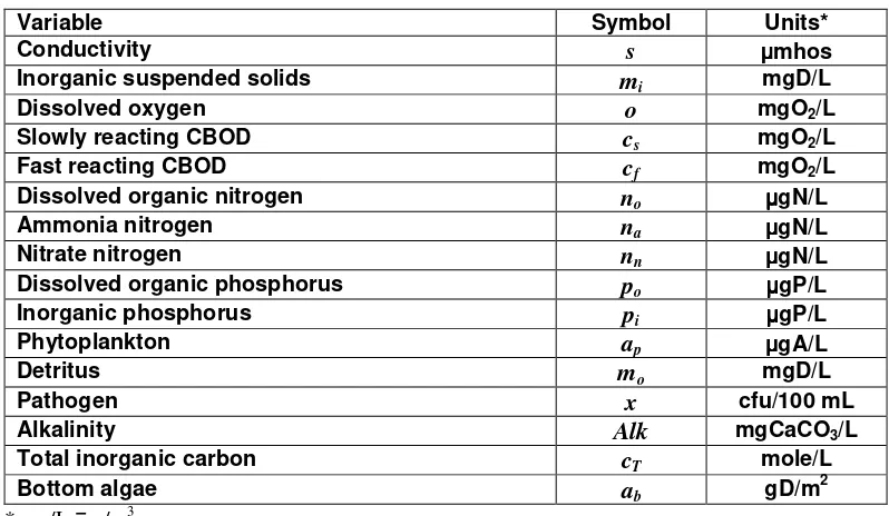
The model constituents are listed in Table 5.

Table 5 Model state variables

Variable Symbol Units*

Conductivity s µµµµmhos

Inorganic suspended solids mi mgD/L

Dissolved oxygen o mgO2/L

Slowly reacting CBOD _cs mgO2/L

Fast reacting CBOD cf mgO2/L

Dissolved organic nitrogen no µµµµgN/L

Ammonia nitrogen na µµµµgN/L

Nitrate nitrogen nn µµµµgN/L

Dissolved organic phosphorus po µµµµgP/L

Inorganic phosphorus pi µµµµgP/L

Phytoplankton _{ap µµµµ}gA/L

Detritus mo mgD/L

Pathogen x cfu/100 mL

Alkalinity Alk mgCaCO3/L

Total inorganic carbon cT mole/L

Bottom algae ab gD/m

2

* mg/L ≡ g/m3

For all but the bottom algae, a general mass balance for a constituent in a reach is written as (Figure 15)

i

inflow outflow

dispersion dispersion

mass load mass abstraction

atmospheric transfer

sediments bottom algae

Figure 15 Mass balance. The external load is computed as

∑

∑

= =

+

=

npsi

j

j npsi j i nps psi

j

j psi j i ps

i

Q

c

Q

c

W

1

, , , 1

, ,

, (56)

where cps,i,j is the jth point source concentration for reach i [mg/L or µg/L], and cnps,i,j is the jth

non-point source concentration for reach i [mg/L or µg/L].

For bottom algae, the transport and loading terms are omitted,

i b i b

S

dt

da

, ,

₌

(57)

where Sb,i = sources and sinks of bottom algae due to reactions [gD/m2/d].

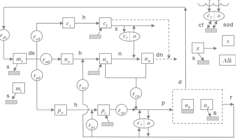
r_cn

Figure 16 Model kinetics and mass transfer processes. The state variables are defined in Table 5. Kinetic processes are dissolution (ds), hydrolysis (h), oxidation (x), nitrification (n), denitrification (dn), photosynthesis (p), death (d), and respiration (r). Mass transfer processes are reaeration (re), settling (s), sediment oxygen demand (SOD), and sediment inorganic carbon flux (cf). Note that the subscript x for the stoichiometric conversions stands for chlorophyll a (a) and dry weight (d) for phytoplankton and bottom algae, respectively.

5.2 Reaction Fundamentals

5.2.1 Biochemical

Reactions

The following chemical equations are used to represent the major biochemical reactions that take place in the model (Stumm and Morgan 1996):

Plant Photosynthesis and Respiration:

Ammonium as substrate:

+

Nitrate as substrate:

Nitrification:

Note that a number of additional reactions are used in the model such as those involved with simulating pH and unionized ammonia. These will be outlined when these topics are discussed later in this document.

5.2.2 Stoichiometry of Organic Matter

The model requires that the stoichiometry of organic matter (i.e., plants and detritus) be specified by the user. The following representation is suggested as a first approximation (Redfield et al. 1963, Chapra 1997),

mgA and A refer to dry weight, carbon, nitrogen, phosphorus, and chlorophyll a, respectively. It should be noted that chlorophyll a is the most variable of these values with a range of approximately 500-2000 mgA (Laws and Chalup 1990, Chapra 1997).

These values are then combined to determine stoichiometric ratios as in

gY gX = xy

r (63)

For example, the amount of nitrogen that is released when 1 gD of detritus is dissolved can be computed as

gD

5.2.2.1 Oxygen Generation and Consumption

The model requires that the rates of oxygen generation and consumption be prescribed. If

ammonia is the substrate, the following ratio (based on Equation 62) can be used to determine the grams of oxygen generated for each gram of plant matter that is produced through photosynthesis.

gC

gC

Note that Equation (68) is also used for the stoichiometry of the amount of oxygen consumed for both plant respiration and fast organic CBOD oxidation.

For nitrification, the following ratio is based on Equation (64)

gN

5.2.2.2 CBOD Utilization Due to Denitrification

As represented by Equation (60), CBOD is utilized during denitrification,

5.2.3 Temperature Effects on Reactions

The temperature effect for all first-order reactions used in the model is represented by

20 the reaction.

5.3 Constituent Reactions

The mathematical relationships that describe the individual reactions and concentrations of the model state variables (Table 5) are presented in the following paragraphs.

5.3.1 Conservative Substance (

s

)

By definition, conservative substances are not subject to reactions:

Ss = 0 (69)

5.3.2 Phytoplankton

(

a

p)

Phytoplankton increase due to photosynthesis. They are lost via respiration, death, and settling

5.3.2.1 Photosynthesis

Phytoplankton photosynthesis is a function of temperature, nutrients, and light

p pa

µ

PhytoPhoto= (71)

where µp = phytoplankton photosynthesis rate [/d], which is calculated as

Lp

nutrient attenuation factor [dimensionless number between 0 and 1], and φLp = the phytoplankton

light attenuation coefficient [dimensionless number between 0 and 1].

Nutrient Limitation. Michaelis-Menten equations are used to represent growth limitation for inorganic nitrogen and phosphorus. The minimum value is then used to compute the nutrient attenuation factor,



where ksNp = nitrogen half-saturation constant [µgN/L] and ksPp = phosphorus half-saturation

constant [µgP/L].

Light Limitation. It is assumed that light attenuation through the water follows the Beer-Lambert law,

where PAR(z) = photosynthetically available radiation (PAR) at depth z below the water surface [ly/d]2, and ke = the light extinction coefficient [m−1]. The PAR at the water surface is assumed to

be a fixed fraction of the solar radiation

)

The extinction coefficient is related to model variables by

3

where keb = the background coefficient accounting for extinction due to water and color [/m], αi,

αo, αp, and αpn, are constants accounting for the impacts of inorganic suspended solids

[L/mgD/m], particulate organic matter [L/mgD/m], and chlorophyll [L/µgA/m and (L/µgA)2/3/m], respectively. Suggested values for these coefficients are listed in Table 6.

2

ly/d = langley per day. A langley is equal to a calorie per square centimeter. Note that a ly/d is related to

Table 6 Suggested values for light extinction coefficients

Symbol Value Reference

αi 0.052 Di Toro (1978)

αo 0.174 Di Toro (1978)

αp 0.0088 Riley (1956)

αpn 0.054 Riley (1956)

Three models are used to characterize the impact of light on phytoplankton photosynthesis (Figure 17):

Figure 17 The three models used for phytoplankton and bottom algae photosynthetic light dependence. The plot shows growth attenuation versus PAR intensity [ly/d]. Half-Saturation (Michaelis-Menten) Light Model:

)

where FLp = phytoplankton growth attenuation due to light and KLp = the phytoplankton light

parameter. In the case of the half-saturation model, the light parameter is a half-saturation coefficient [ly/d]. This function can be combined with the Beer-Lambert law and integrated over water depth, H [m], to yield the phytoplankton light attenuation coefficient



Smith’s Function:

where KLp = the Smith parameter for phytoplankton [ly/d]; that is, the PAR at which growth is

70.7% of the maximum. This function can be combined with the Beer-Lambert law and integrated over water depth to yield

Steele’s Equation:

Lp

where KLp = the PAR at which phytoplankton growth is optimal [ly/d]. This function can be

combined with the Beer-Lambert law and integrated over water depth to yield



5.3.2.2 Losses

Respiration. Phytoplankton respiration is represented as a first-order rate that is attenuated at low oxygen concentration,

p rp T a k ( )

PhytoResp= (83)

where krp(T) = temperature-dependent phytoplankton respiration rate [/d].

Death. Phytoplankton death is represented as a first-order rate,

p dp T a k ( )

PhytoDeath= (84)

where kdp(T) = temperature-dependent phytoplankton death rate [/d].

Settling. Phytoplankton settling is represented as

p a _a H v

PhytoSettl= (85)

where va = phytoplankton settling velocity [m/d].

5.3.3 Bottom algae (

a

b

)

h BotAlgDeat BotAlgResp

o

BotAlgPhot − −

= ab

S (86)

5.3.3.1 Photosynthesis

The representation of bottom algae photosynthesis is a simplification of a model developed by Rutherford et al. (1999). Photosynthesis is based on a temperature-corrected zero-order rate attenuated by nutrient and light limitation,

Lb Nb gb T C ( )φ φ o

BotAlgPhot = (87)

where Cgb(T) = the temperature-dependent maximum photosynthesis rate [gD/(m2 d)],φNb =

bottom algae nutrient attenuation factor [dimensionless number between 0 and 1], and φLb = the

bottom algae light attenuation coefficient [dimensionless number between 0 and 1].

Temperature Effect. As for the first-order rates, an Arrhenius model is employed to quantify the effect of temperature on bottom algae photosynthesis,

20

Nutrient Limitation. Michaelis-Menten equations are used to represent growth limitation due to inorganic nitrogen and phosphorus. The minimum value is then used to compute the nutrient attenuation coefficient,

where ksNb = nitrogen half-saturation constant [µgN/L] and ksPb = phosphorus half-saturation

constant [µgP/L].

Light Limitation. In contrast to the phytoplankton, light limitation at any time is determined by the amount of PAR reaching the bottom of the water column. This quantity is computed with the Beer-Lambert law (recall Equation 78) evaluated at the bottom of the river,

H

As with the phytoplankton, three models (Equations 81, 83, and 85) are used to characterize the impact of light on bottom algae photosynthesis. Substituting Equation (97) into these models yields the following formulas for the bottom algae light attenuation coefficient,

Half-Saturation Light Model:

H

(

)

2

Steele’s Equation:

Lb

where KLb = the appropriate bottom algae light parameter for each light model.

5.3.3.2 Losses

Respiration. Bottom algae respiration is represented as a first-order rate that is attenuated at low oxygen concentration,

b rb T a k ( )

BotAlgResp= (94)

where krb(T) = temperature-dependent bottom algae respiration rate [/d].

Death. Bottom algae death is represented as a first-order rate,

b db T a k ( ) h

BotAlgDeat = (95)

where kdb(T) = the temperature-dependent bottom algae death rate [/d].

5.3.4 Detritus

(

m

o

)

Detritus or particulate organic matter (POM) increases due to plant death. It is lost via dissolution and settling

where kdt(T) = the temperature-dependent detritus dissolution rate [/d] and

o dt _m H v

DetrSettl= (98)

5.3.5 Slowly Reacting CBOD (

c

s

)

Slowly reacting CBOD increases due to detritus dissolution. It is lost via hydrolysis.

SlowCHydr DetrDiss−

= od cs r

S (99)

where

s hc T c k ( )

SlowCHydr = (100)

where khc(T) = the temperature-dependent slow CBOD hydrolysis rate [/d].

5.3.6 Fast Reacting CBOD (

c

f

)

Fast reacting CBOD is gained via the hydrolysis of slowly-reacting CBOD. It is lost via oxidation and denitrification.

Denitr Oxid

FastC

SlowCHydr _ondn

cf r

S = − − (101)

where

f dc oxcf k T c F ( )

FastCOxid= (102)

where kdc(T) = the temperature-dependent fast CBOD oxidation rate [/d] and Foxcf = attenuation

due to low oxygen [dimensionless]. The parameter rondn is the ratio of oxygen equivalents lost per

nitrate nitrogen that is denitrified (Equation 71). The term Denitr is the rate of denitrification [µgN/L/d]. It will be defined in 5.3.10 below.

Three formulations are used to represent the oxygen attenuation:

Half-Saturation:

o K

o F

socf

oxrp = ₊ (103)

where Ksocf = half-saturation constant for the effect of oxygen on fast CBOD oxidation [mgO2/L].

Exponential:

) 1

( K o

oxrp e socf

F = − − (104)

where Ksocf = exponential coefficient for the effect of oxygen on fast CBOD oxidation [L/mgO2].

2

where Ksocf = half-saturation constant for second-order effect of oxygen on fast CBOD oxidation

[mgO22/L2].

5.3.7 Dissolved Organic Nitrogen (

n

o)

Dissolved organic nitrogen increases due to detritus dissolution. It is lost via hydrolysis.

DONHydr

where khn(T) = the temperature-dependent organic nitrogen hydrolysis rate [/d].

5.3.8 Ammonia Nitrogen (

n

a)

Ammonia nitrogen increases due to dissolved organic nitrogen hydrolysis and plant respiration. It is lost via nitrification and plant photosynthesis:

o

The ammonia nitrification rate is computed as

a n oxnak T n F ( )

NH4Nitrif= (109)

where kn(T) = the temperature-dependent nitrification rate for ammonia nitrogen [/d] and Foxna =

attenuation due to low oxygen [dimensionless]. Oxygen attenuation is modeled by Equations (106) to (108) with the oxygen dependency represented by the parameter Ksona.

The coefficients Pap and Pap are the preferences for ammonium as a nitrogen source for

phytoplankton and bottom algae, respectively,

)

where khnxp = preference coefficient of phytoplankton for ammonium [mgN/m3] and khnxb =

5.3.9 Unionized

Ammonia

The model simulates total ammonia. In water, the total ammonia consists of two forms: ammonium ion, NH4+, and unionized ammonia, NH3. At normal pH (6 to 8), most of the total

ammonia will be in the ionic form. However at high pH, unionized ammonia predominates. The amount of unionized ammonia can be computed as

a u au

F

n

n

=

(112)

where nau = the concentration of unionized ammonia [µgN/L], and Fu = the fraction of the total

ammonia that is in unionized form,

a

where Ka = the equilibrium coefficient for the ammonia dissociation reaction, which is related to

temperature by

a

Nitrate nitrogen increases due to nitrification of ammonia. It is lost via denitrification and plant photosynthesis:

The denitrification rate is computed as

n

where kdn(T) = the temperature-dependent denitrification rate of nitrate nitrogen [/d] and Foxdn =

effect of low oxygen on denitrification [dimensionless] as modeled by Equations (106) to (108) with the oxygen dependency represented by the parameter Ksodn.

5.3.11 Dissolved Organic Phosphorus (

p

o

)

Dissolved organic phosphorus increases due to dissolution of detritus. It is lost via hydrolysis.

DOPHydr DetrDiss−

= pd po r

where

o hp T p k ( )

DOPHydr = (118)

where khp(T) = the temperature-dependent organic phosphorus hydrolysis rate [/d].

5.3.12 Inorganic Phosphorus (

p

i

)

Inorganic phosphorus increases due to dissolved organic phosphorus hydrolysis and plant respiration. It is lost via plant photosynthesis:

o

5.3.13 Inorganic Suspended Solids (

m

i

)

Inorganic suspended solids are lost via settling,

Smi = – InorgSettl

InorgSettl= (120)

where vi = inorganic suspended solids settling velocity [m/d].

5.3.14 Dissolved Oxygen (

o

)

Dissolved oxygen increases due to plant photosynthesis. It is lost via fast CBOD oxidation, nitrification and plant respiration. Depending on whether the water is undersaturated or oversaturated it is gained or lost via reaeration,

OxReaer

OxReaer

(122)

where ka(T) = the temperature-dependent oxygen reaeration coefficient [/d], os(T, elev) = the

saturation concentration of oxygen [mgO2/L] at temperature, T, and elevation above sea level,

5.3.14.1 Oxygen Saturation

The following equation is used to represent the dependence of oxygen saturation on temperature (APHA 1992)

where o_s(T, 0) = the saturation concentration of dissolved oxygen in freshwater at 1 atm [mgO2/L]

and T_a = absolute temperature [K] where Ta = T +273.15.

The effect of elevation is accounted for by

)

5.3.14.2 Reaeration Formulas

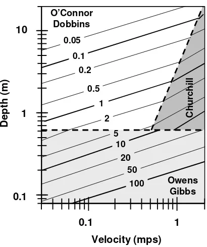
The reaeration coefficient can be prescribed on the Reach worksheet. If reaeration is not prescribed, it can be computed using one of the following formulas:

O’Connor-Dobbins:

Reaeration can also be internally calculated based on the following scheme patterned after a plot developed by Covar (1976) (Figure 18):

If H > 0.61 m and H > 3.45U2.5, use the O’Connor-Dobbins formula

Otherwise, use the Churchill formula

This is referred to as option Internal on the Rates worksheet of Q2K.

0.1 1 10

D

e

pt

h (

m

)

0.1 1

Velocity (mps)

Owens Gibbs 10

100 O’Connor

Dobbins

0.1

1 0.2

0.5

C

hur

chi

ll

0.05

2

20 50 5

Figure 18 Reaeration rate (/d) versus depth and velocity (Covar 1976).

5.3.14.3 Effect of Control Structures: Oxygen

Oxygen transfer in streams is influenced by the presence of control structures such as weirs, dams, locks, and waterfalls (Figure 19). Butts and Evans (1983) have reviewed efforts to characterize this transfer and have suggested the following formula,

)

046

.

0

1

)(

11

.

0

1

(

38

.

0

1

a

b

H

H

T

r

_d

=

+

_{d d d}

−

_d

+

(128)

where rd = the ratio of the deficit above and below the dam, Hd = the difference in water elevation

[m] as calculated with Equation (7), T = water temperature (°C) and ad and bd are coefficients that

correct for water-quality and dam-type. Values of these coefficients are summarized in Table 7.

Q

_{i−−−−1}

o’

_{i−−−−1}

H

_d

Q

_{i−−−−1}

o

_{i−−−−1}

Figure 19 Water flowing over a river control structure.

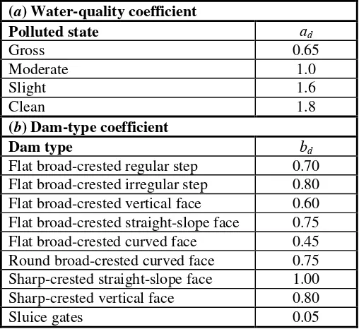
Table 7 Coefficient values used to predict the effect of dams on stream reaeration.

(a) Water-quality coefficient

Polluted state ad

Gross 0.65

Moderate 1.0

Slight 1.6

Clean 1.8

(b) Dam-type coefficient

Dam type bd

Flat broad-crested regular step 0.70 Flat broad-crested irregular step 0.80 Flat broad-crested vertical face 0.60 Flat broad-crested straight-slope face 0.75 Flat broad-crested curved face 0.45 Round broad-crested curved face 0.75 Sharp-crested straight-slope face 1.00

Sharp-crested vertical face 0.80

Sluice gates 0.05

The oxygen mass balance for the reach below the structure is written as

(

)

oi

Pathogens are subject to death and settling,

PathSettl PathDeath −

− = x

S (131)

5.3.15.1 Death

(

e

)

x

where kdx(T) = temperature-dependent pathogen die-off rate [/d].

5.3.15.2 Settling

Pathogen settling is represented as

x H v_x

PathSettl= (133)

where vx = pathogen settling velocity [m/d].

5.3.16 pH

The following equilibrium, mass balance and electroneutrality equations define a freshwater dominated by inorganic carbon (Stumm and Morgan 1996),

]

dissolved carbon dioxide and carbonic acid, HCO3− = bicarbonate ion, CO3 2−

= carbonate ion, H+ = hydronium ion, OH− = hydroxyl ion, and cT = total inorganic carbon concentration [mole L−

1

]. The brackets [ ] designate molar concentrations.

Note that the alkalinity is expressed in units of eq/L for the internal calculations. For input and output, it is expressed as mgCaCO3/L. The two units are related by

eq/L)

The equilibrium constants are corrected for temperature by

80

Plummer and Busenberg (1982):

2

Plummer and Busenberg (1982):

2

The nonlinear system of five simultaneous equations (138 through 142) can be solved numerically for the five unknowns: [H2CO3*], [HCO3−], [CO3

2−

], [OH−], and {H+}. As presented Stumm and Morgan (1996), an efficient solution method can be derived by combining Equations (138), (139) and (141) to define the quantities (Stumm and Morgan 1996)

2

carbonate, respectively. Equations (140), (142), (148) and (149) can then be combined to yield,

]

Thus, solving for pH reduces to determining the root, {H+}, of

Alk

where pH is then calculated with

] H [ log

pH=− ₁₀ + (148)

The root of Equation (151) is determined with the bisection method (Chapra and Canale 2002).

Total inorganic carbon concentration increases due to fast carbon oxidation and plant respiration. It is lost via plant photosynthesis. Depending on whether the water is undersaturated or

oversaturated with CO2, it is gained or lost via reaeration,

CO2Reaer

where kac(T) = the temperature-dependent carbon dioxide reaeration coefficient [/d], and [CO2]s =

the saturation concentration of carbon dioxide [mole/L].

The stoichiometric coefficients are derived from Equation (62)3

L

5.3.17.1 Carbon Dioxide Saturation

The CO2 saturation is computed with Henry’s law,

2

CO2 = the partial pressure of carbon dioxide in

the atmosphere [atm]. Note that users input the partial pressure to Q2K in ppm. The program internally converts ppm to atm using the conversion: 10−6 atm/ppm.

The value of K_H can be computed as a function of temperature by (Edmond and Gieskes 1970)

The conversion, m3 = 1000 L is included because all mass balances express volume in m3, whereas total

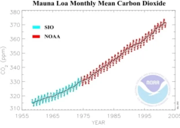
The partial pressure of CO₂ in the atmosphere has been increasing, largely due to the combustion of fossil fuels (Figure 20). Values in 2003 are approximately 10-3.43 _{atm (= 372 ppm).}

Figure 20 Concentration of carbon dioxide in the atmosphere as recorded at Mauna Loa Observatory, Hawaii. (http://www.cmdl.noaa.gov/ccg/figures/co2mm_mlo.jpg).

5.3.17.2 CO2 Gas Transfer

The CO2 reaeration coefficient can be computed from the oxygen reaeration rate by

)

5.3.17.3 Effect of Control Structures: CO2

As was the case for dissolved oxygen, carbon dioxide gas transfer in streams can be influenced by the presence of control structures. Q2K assumes that carbon dioxide behaves similarly to

dissolved oxygen (recall Sec. 5.3.14.3). Thus, the inorganic carbon mass balance for the reach immediately downstream of the structure is written as

(

)

cTi

d

where rd is calculated with Equation (132).

5.3.18 Alkalinity (Alk)

The present model accounts for changes in alkalinity due to plant photosynthesis and respiration, nitrification, and denitrification.

(

)

where the r’s are ratios that translate the processes into the corresponding amount of alkalinity. The stoichiometric coefficients are derived from Equations (62) through (65) as in

Phytoplankton Photosynthesis (Ammonia as Substrate) and Respiration:

L

Phytoplankton Photosynthesis (Nitrate as Substrate):

L

Bottom Algae Photosynthesis (Ammonia as Substrate) and Respiration:

L

Bottom Algae Photosynthesis (Nitrate as Substrate):

L 1000

m 1 mgN 1000

gN 1 gN 14 moleN moleN

1 eqH

4 _{× × ×} 3

= +

alkden

r (165)

5.4 SOD/Nutrient Flux Model

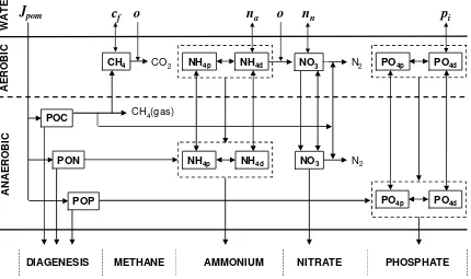
Sediment nutrient fluxes and sediment oxygen demand (SOD) are based on a model developed by Di Toro (Di Toro et al. 1991, Di Toro and Fitzpatrick. 1993, Di Toro 2001). The present version also benefited from James Martin’s (Mississippi State University, personal communication) efforts to incorporate the Di Toro approach into EPA’s WASP modeling framework.

A schematic of the model is depicted in Figure 21. As can be seen, the approach allows oxygen and nutrient sediment-water fluxes to be computed based on the downward flux of particulate organic matter from the overlying water. The sediments are divided into 2 layers: a thin (≅ 1 mm) surface aerobic layer underlain by a thicker (10 cm) lower anaerobic layer. Organic carbon, nitrogen and phosphorus are delivered to the anaerobic sediments via the settling of particulate organic matter (i.e., phytoplankton and detritus). There they are transformed by mineralization reactions into dissolved methane, ammonium and inorganic phosphorus. These constituents are then transported to the aerobic layer where some of the methane and ammonium are oxidized. The flux of oxygen from the water required for these oxidations is the sediment oxygen demand. The following sections provide details on how the model computes this SOD along with the sediment-water fluxes of carbon, nitrogen and phosphorus that are also generated in the process.

CH4 NO3

NO3

NH4d PO4p PO4d

NH4p NH4d

PO4p PO4d

CO₂ N₂

N₂

POC

c

_f

o

n

_a

o

n

_n

p

_i

J

_pom

NH4p

CH4(gas)

POP

DIAGENESIS METHANE AMMONIUM NITRATE PHOSPHATE

AE

RO

B

IC

A

N

A

E

ROBIC

WA

T

E

R

PON