ABSTRACT:
Reliable obstacle avoidance is a key to navigating with UAVs in the close vicinity of static and dynamic obstacles. Wheel-based mobile robots are often equipped with 2D or 3D laser range finders that cover the 2D workspace sufficiently accurate and at a high rate. Micro UAV platforms operate in a 3D environment, but the restricted payload prohibits the use of fast state-of-the-art 3D sensors. Thus, perception of small obstacles is often only possible in the vicinity of the UAV and a fast collision avoidance system is necessary. We propose a reactive collision avoidance system based on artificial potential fields, that takes the special dynamics of UAVs into account by predicting the influence of obstacles on the estimated trajectory in the near future using a learned motion model. Experimental evaluation shows that the prediction leads to smoother trajectories and allows to navigate collision-free through passageways.
1 INTRODUCTION
We aim for fully autonomous geometric and semantic mapping of (partially) unknown environments using a multicopter based on the MikroKopter platform (MikroKopter, 2013). This high-level task demands detailed flight plans that fulfill the mission objectives and ensure collision-free navigation in the vicinity of buildings, vegetation, and dynamic obstacles. Due to the com-plex flight dynamics of the unmanned aerial vehicle (UAV) and dynamic or previously unknown obstacles, it is necessary for the UAV to quickly react on deviations from the plan. For this pur-pose we follow a multi-layer approach for the navigation of the UAV. Within the lower layers, high-frequency controllers stabi-lize the attitude of the multicopter. A control layer provides an interface to the higher layers, allowing control of linear and an-gular velocities instead of the multicopter’s attitude and thrust. Between the control and the higher planning layers (3D path and mission planning), we employ a fast reactive collision avoidance module based on artificial potential fields (Ge and Cui, 2002). We have chosen this approach as a safety measure reacting di-rectly on the available sensor information at a higher frequency than used for planning. This enables the UAV to immediately react to perceived obstacles in its vicinity. Furthermore, it can handle small deviations from the planned path caused by external influences such as wind without raising the need to costly replan-ning on higher planreplan-ning layers. Also in manual operation, obsta-cle avoidance assists a human pilot to operate the UAV safely in challenging situations, e. g., flying through a narrow passageway.
We take the special properties of UAVs in contrast to earthbound vehicles into account, by extending the classic potential field ap-proach to collision avoidance with a prediction of the outcome of a chosen control for a fixed time horizon. This improves the navigation performance and closes the gap between pure reactive control and planned motions.
After a discussion of related work in the next section, we will briefly describe our UAV’s motion control architecture. In Sec. 4 we detail our potential field-based approach to collision avoid-ance. The used motion model is explained in Sec. 5. We give an overview over our simulation environment and report results from simulation and a proof of concept example on the real UAV in Sec. 6. Finally, we conclude our paper and discuss future work.
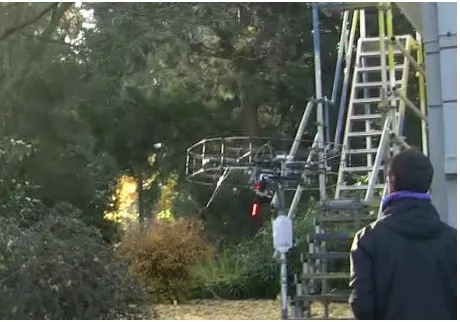
Figure 1: Our local obstacle avoidance algorithm acts as a safety measure between control inputs given by a planning layer or a human pilot remotely controlling the robot. This ensures safe operation in challenging situations, e. g., narrow passageways.
2 RELATED WORK
The application of UAVs in recent robotics research varies es-pecially in the level of autonomy ranging from basic hovering and position holding (Bouabdallah et al., 2004) over trajectory tracking and waypoint navigation (Puls et al., 2009) to fully au-tonomous navigation (Grzonka et al., 2012).
Particularly important for fully autonomous operation is the abil-ity to perceive obstacles and avoid collisions. Obstacle avoidance is often neglected, e. g., by flying in a certain height when au-tonomously flying between waypoints. Most approaches to ob-stacle avoidance for micro UAVs are camera-based due to the constrained payload (Mori and Scherer, 2013, Ross et al., 2013). Hence, collision avoidance is restricted to the narrow field of view (FoV) of the cameras.
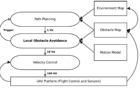
Figure 2: The control concept of our UAV is a hierarchical trol architecture with planning layers on the top and faster con-trol layers on the bottom. A path planner ensures the planning completeness, a fast obstacle avoidance layer selects appropriate velocity commands. These are fed to low-level controllers to con-trol the UAV. Commands are depicted by solid lines, data flow is depicted by dotted lines.
camera pair (facing forwards), and the 2D measurement plane of the scanner when flying sideways. They do not perceive obstacles outside of this region or behind the vehicle.
We allow omnidirectional movements of our UAV, thus we have to take obstacles in all directions of the UAV into account. Our main sensor for omnidirectional obstacle perception is a lightweight rotating 3D laser scanner based on a Hokuyo UTM-30LX-EW 2D LRF. Furthermore, we augment our obstacle map with visu-ally perceived objects from two wide-angle stereo cameras. To perceive smaller objects, or objects that optical sensors cannot perceive reliably, we installed a ring of eight ultra sonic sensors covering the volume around our UAV. For a detailed description of our sensor setup and the processing pipeline see (Holz et al., 2013, Droeschel et al., 2013). Another micro UAV with a sensor setup that allows omnidirectional obstacle perception is described in (Chambers et al., 2011).
A two-level approach to collision-free navigation using artificial potential fields on the lower layer is proposed in (Ok et al., 2013). Similar to our work, completeness of the path planner is guaran-teed by a layer on top of local collision avoidance. In contrast to this work, we consider the current motion state of the UAV and select motion commands accordingly.
Some other reactive collision avoidance algorithms for UAVs are based on optical flow (Green and Oh, 2008) or a combination of flow and stereo vision (Hrabar et al., 2005). However, solely op-tical flow-based solutions cannot cope well with frontal obstacles and these methods are not well suited for omnidirectional obsta-cle avoidance as needed for our scenario.
Recent search-based methods for obstacle-free navigation include (MacAllister et al., 2013, Cover et al., 2013). A good survey on approaches to motion planning for UAVs is given in (Goerzen et al., 2010). These methods assume complete knowledge of the scene geometry, an assumption that we do not make here.
3 CONTROL ARCHITECTURE
We designed a hierarchical control architecture for our UAV, with high-frequency controllers on the lower layers and slower plan-ners on the upper layers, that solve more complex path and mis-sion planning problems at a lower frequency (see Fig. 2). In this
Figure 3: We discretize our UAV into cells (blue) and calculate the forces per cell. The artificial force applied to the UAV is the average of all forces. The nearest obstacles to the cells are depicted by red lines.
paper, we abstract the planning layers as a black box providing the lower layer with globally consistent paths given a static envi-ronment model and the local obstacle map. The provided trajec-tories serve as input for the local collision avoidance layer, that we will detail in the next section. Due to the reactive nature and restricted information about the environment, the local collision avoidance can get stuck in local minima. In this case, a failure condition is detected and a global path planner has to be triggered to generate a new valid trajectory.
The local obstacle avoidance commands ego-centric linear veloc-ities to the low-level control layer at a rate of10 Hz. The UAVs onboard hardware controllers control the attitude of the vehicle according to measurements of an onboard inertial measurement unit (IMU). The attitude is closely related to the acceleration of the UAV (c.f. Sec. 5), but small measurement errors of the IMU and other sources of acceleration like the air flow render simple integration over time to estimate the UAVs velocity infeasible. Hence, we added another control layer between the local obsta-cle avoidance and the hardware controller, that controls the UAVs attitude according to a commanded linear velocity setpoint. We employ decoupled PID controllers for each element of the four di-mensional setpoint(vx, vy, vz, ω). The controlled motion state is
estimated by an extended Kalman Filter (EKF) and observations from multiple sources, i. e., IMU data, optical flow (Honegger et al., 2013), visual odometry (Klein and Murray, 2007), GPS, and possibly other external sources, like a motion capture sys-tem, depending on the availability. A motion model can be used to predict away the control latencies.
4 LOCAL OBSTACLE AVOIDANCE
The major design goal of our approach to obstacle avoidance is to react quickly on newly perceived obstacles. For this purpose, we extend artificial potential fields as these can be evaluated at the same frequency as new sensor data is processed. Furthermore, even in cases where it becomes infeasible to determine a valid trajectory to an intermediate goal or a collision is inevitable, the resulting control command will avoid obstacles or at least decel-erate the UAV, in the later case.
As input for our algorithm, we consider a robot-centered 3D oc-cupancy grid, the current motion statext, and a target waypoint
wt on a globally planned 3D path. In detail, the 3D occupancy
goal. The waypoint is selected from a globally planned path in a way that avoids the reactive approach to get stuck in a lo-cal minimum. The perceived obstacles induce repulsive forces on the flying robot. The magnitude of the repulsive force Fr
of the closest obstacleoat a positionpis calculated asFr,p =
costs (argmino(ko−pk)), where costs is a function that is
zero in a user-defined safe distance to obstacles and raises with decreasing distance. This yields a repulsive force vectorF~r,p =
Fr,pkpp−−ook.
The resulting force at a discrete position is now the weighted sum of the attractive and repulsive forcesFp=aFa,p+bFr,p, with
user-defined weighting factorsa, b. A 2D example of the result-ing potential field is depicted in Fig. 4.
As most of the cells in our obstacle map are free space, we do not pre-calculate the forces for every cell, but only for cells that intersect with the robot’s bounding box. Due to the discrete na-ture of our algorithm, we split the robot’s bounding box into cells matching the size of a cell in our obstacle map. The resulting force applied to the robot is the average of all forces applied to the center points of these cells (see Fig. 3). Thus, we do not need to enlarge obstacles and avoid oscillations caused by the discretization. The motion command sent to the robot’s low-level controller is calculated according to the resulting artificial forces.
In contrast to the idealized massless particle assumed in the po-tential field approach, frequent acceleration and deceleration of the UAV to follow the most cost-efficient path through the field is disadvantageous. To be able to totally change the motion di-rection at every discrete position would require low velocities. Hence, we accept suboptimal paths, as long as they do not lead to a motion state that will cause a collision in the future, e. g., if the UAV becomes too fast in the vicinity of obstacles. To account for the dynamic statextof the UAV, we predict the robot’s future
tra-jectoryTtgiven the current linear velocitiesvt, the attitudeRt,
and the probable sequence of motion commandsut:t+ngiven in
the nextntime steps (Fig. 5). To predict the trajectory, we em-ploy a learned motion model of the UAV (c.f. Sec. 5) and the expected resulting forces along the trajectory, given the current knowledge about the world.
These predicted forces are used to influence the motion command selection. Larger forces indicate that the UAV will come close to an obstacle in the future while following the trajectory started by the current motion command. Hence, the next velocity com-manded to the low-level controller needs to be reduced, accord-ingly. This is implemented in our algorithm as a reduction of the maximum velocity for the next motion command, if the magni-tude of the forces along the trajectory becomes too large. For the prediction of the trajectory, this new maximum velocity is as-sumed as the maximum in the predicted future.
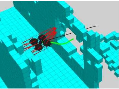
Figure 5: We predict the influence of a motion command by rolling out the robot’s trajectory (green) using a learned motion model. The current artificial repulsive forces are depicted in red.
The prediction of the trajectoryTtis implemented as follows
Tt = pt:t+n= (pt, pt+ 1, . . . , pt+n)
pi+1 = Axi+Bui+pi i∈[t:t+n−1]
ui = C ~Fpi,
where A, B denote matrices based on our motion model (de-scribed in the next section) to estimate a pose difference given the dynamic state and a control input. C denotes a mapping of a force vector to a velocity command. Given the estimated se-quence of future positionspt:t+n, we search the smallest index
i ∈ (t:t+n)for which the magnitude of the force exceeds a threshold, i. e.,Fpi > Fmax. If such aniexists, we reduce the
maximum velocityvmaxto
vnew=
1 2+
i
2n
vmax.
Hence, while approaching an obstacle the maximum velocity com-manded to the UAV is gradually reduced.
In the case that no trajectory with sufficiently small predicted forces can be found, the UAV stops. Here, we exploit the property of multicopters that, in contrast to fixed-wing UAVs, the dynamic state of the system can be changed completely within a short time. Hence, the look-ahead needed to estimate the effects of a control input is tightly bound. We have chosen the length of the trajec-tory roll out as the time the multicopter needs to stop, which is one second.
5 LEARNING A MOTION MODEL
To obtain a motion model of our robot we fly our multicopter re-mote controlled within a motion capture system (MoCap). This system provides ground-truth data of the robot’s position and at-titude at an average rate of 100 Hz allowing for the derivation of the robot’s dynamic state. Due to inconsistent delays within the MoCap system, captured data is often noisy and unsuitable for simple delta-time differentiation needed to correctly calculate the dynamic state. Thus after capturing, all data is processed using a low-pass filter allowing for more accurate estimates of instanta-neous velocities.
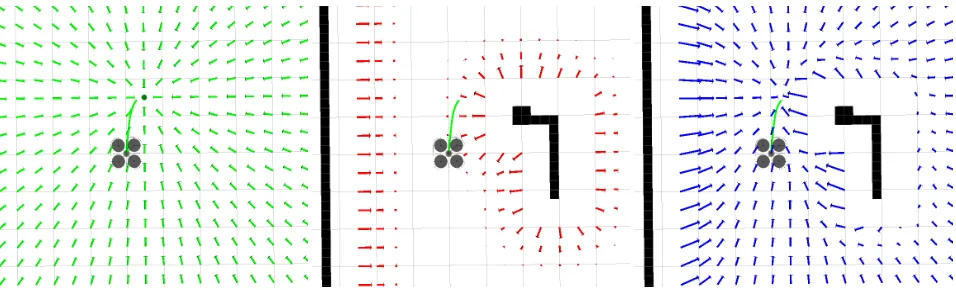
Figure 4: The robot’s local trajectory (green) is influenced by a weighted sum of attractive (left) and repulsive forces (middle). This induces an artificial potential field to navigate collision-free to an intermediate goal (right).
of the data capturing system, these two components are initially captured using different computer system and later fused. As timestamps rarely coincide, interpolation of the filtered state is matched with control commands and transformed from the ”cap-ture frame” into the ”UAV frame” while scaling the control com-mands to a[−1,1]scale. The final state estimate data can be used to derive the motion model parameters.
Several effects from flying within the MoCap system must be considered before an appropriate motion model can be derived. Due to a restricted capture volume, external thrust effects can be observed due to ground, ceiling, and wall planes interacting with the propeller-generated wind. These effects are minimized when flying within the central region of the capture volume, thus data acquisition is only performed within this restricted volume. Ad-ditionally, some maneuvers are impossible to capture due to both safety and acceleration constraints - however as flying advanced maneuvers is not a goal of the project, this issue can be safely ignored. Using this simple set of capture constraints, external factors to the motion of the multicopter can be minimized.
We model the flight dynamics as a time-discrete linear dynamic system (LDS)xt+1 =Axt+Butthat predicts the state of the
UAV at the timet+ 1given the current state estimatext(i.e.
at-titudeRt, positionpt, angularωtand linearvtvelocities, thrust
Tt) and the user command inputut. The state transition model
Aand control-input modelBare fitted to the captured data using ordinary least squares. Due to the properties of a multicopter and through repeated verification using the MoCap system, the atti-tude in the horizontal plane (i.e. roll and pitch) when maintaining altitude is assumed to be proportional to the acceleration along the corresponding axis. Additionally, the yaw component of the model is considered independent from the remaining parameters.
Considering only the horizontal plane velocity and attitude (i.e. x and y axes), the transition modelAfor the x and y axis velocities has the general form:
whereDijrepresents the dampening effects in thei-axis given
the j-axis velocity andAij represents the acceleration effects
from attitude in the i-axis given thej-axis attitude. Generally the dampening termsDxx,Dyyare near1;Dxy,Dyxare near0
while the acceleration termsAxy,Ayxcorrespond to the
propor-tionality constant of the attitude;Axx,Ayyare near0(note that
an attitude in one axis affects the acceleration of the perpendicu-lar axis). Additionally, due to a non-symmetric inertia tensor of
the multicopter, these matrix values may also not be symmetric resulting in different accelerations and dampening for the forward and lateral movements. The reduced state input consists of the x and y axis velocity (Vx,Vy) and the x and y axis rotations
corre-sponding to roll and pitch, respectively (Rx,Ry).
Through similar analysis, the control-input modelBin the hori-zontal plane velocity and attitude (x and y axes) has the general form:
with control inputut=
αx
αy
whereΦAij represents the integrated accelerations from control
input angles over the time period used for model learning in thei axis from control inputj.δijapproximates the reaction constants
of the multicopter system to reach a desired attitude in theiaxis from the jaxis desired input. The control input is the desired attitude for thexandy axes (i.e. roll and pitch respectively). BothΦAxαx,ΦAyαy are relatively large whileΦAxαy,ΦAyαx
are small showing a independence between multicopter rotation axes. Theδvalues also show an independence between rotation axes, however their values are specific to both the multicopter control reaction speed, control delay, thrust output, and time pe-riod used for learning.
In addition to predicting the trajectory for the purpose of colli-sion avoidance, this model can be utilized in the low-level ve-locity controller (Achtelik et al., 2009), for kinodynamic motion planning (S¸ucan and Kavraki, 2009), and to predict away system delays due to the time difference of control input and control exe-cution. Furthermore, our simulation environment uses the model to ensure realistic behavior of the simulated multicopter.
6 EVALUATION
We evaluate the accuracy of our learned motion model and the performance and reliability of our predictive collision avoidance module in simulation and on the real system.
6.1 Simulation Environment
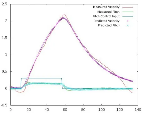
Figure 6: Example of a learned motion model. We compared the predicted pitch angle and resulting linear velocity (crosses) given an user input with the measured ground-truth data (lines).
at simulating flying robots. Hence, we extended the simulator to move objects according to a black box motion model, given exter-nal control inputs and timings from simulation. Here, we can use learned motion models of a UAV as plugins to move them realis-tic, without loosing other capabilities of the simulator like simu-lated sensors or collision detection. Furthermore, we developed modules to support multi-echo laser range finders (e. g., Hokuyo UTM-30LX-EW) and ultra sonic sensors.
6.2 Experiments
We tested our approach in waypoint following scenarios in sim-ulation. The tests include bounded environments with walls and unbounded environments, where the waypoints direct the UAV through window like openings of different size. These experi-ments revealed that our collision avoidance approach is able to follow paths, if a relatively sparse trajectory is given that cov-ers the most crucial navigation points. The simulated UAV was able to fly through all passageways and windows of its size plus a safety margin (see Fig. 5). The prediction of the near future out-come of motion commands leads to smoother trajectories, keep-ing the UAV further away from obstacles than the same potential field approach without trajectory prediction while allowing com-parable velocities as the classic approach.
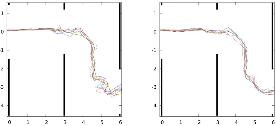
We compared our approach with a classic potential field approach without look-ahead in a scenario containing several walls with window-like openings of different size. Furthermore, we evalu-ated the effect of a fixed reduction of the velocity with and with-out trajectory prediction, i. e., reduced velocity if a force thresh-old is reached now or in the predicted time horizon, respectively. Example trajectories from the test runs are depicted in Fig. 7. We summarize the average repulsive forces, a measure of the prox-imity of obstacles during a flight, and the average durations of the test runs in Tab. 1. No collisions occurred during these test runs. Experiments with the real system have shown that the hovering multicopter can avoid approaching obstacles.
We evaluated the learned motion model by comparing the propa-gated dynamic state of an UAV given an user input with ground truth data from the MoCap (Fig. 6). The predicted state of the UAV matches the real state well for time periods sufficiently long for our predictive approach.
Our collision avoidance approach runs at approximately 100 Hz on a single core of an Intel Core 2 processor, which includes data
acquisition and map building. Hence, this collision avoidance al-gorithm is particularly well suited for UAVs with relatively small processing power or complex scenarios where the onboard com-pute unit has to carry out many other processing tasks in parallel.
7 CONCLUSIONS
We developed a fast, reactive collision avoidance layer to quickly react on new measurements of nearby obstacles. It serves as a safety measure between higher planning layers or commands given by a human pilot and the low-level control layer of the UAV. Standard potential field approaches assume that the motion of a vehicle can be changed immediately at any position in the field. To overcome this limitation, we predict the trajectory resulting from the current dynamic state and the artificial potential field into the future. This leads to safer and smoother trajectories for a multicopter. To predict the UAV’s trajectory we employ learned motion models.
In future work, we will focus on the high-level planning layers, to plan qualitatively good, globally consistent, paths at a rate of
1 Hzor faster, to avoid local minima and to accomplish the mis-sion goals in an optimal way. Therefore, we will employ mul-tiresolution path planning techniques (Behnke, 2004), that we will transfer from earthbound robots to UAVs. Furthermore, we will investigate the possibility to learn motion models outside of a MoCap system using precise differential GPS and IMU data.
ACKNOWLEDGMENTS
This work has been supported partially by grant BE 2556/8-1 of German Research Foundation (DFG).
REFERENCES
Achtelik, M., Bachrach, A., He, R., Prentice, S. and Roy, N., 2009. Autonomous navigation and exploration of a quadrotor he-licopter in GPS-denied indoor environments. In: Proceedings of the IEEE International Conference on Robotics and Automation (ICRA).
Behnke, S., 2004. Local multiresolution path planning. Robocup 2003: Robot Soccer World Cup VII pp. 332–343.
Bouabdallah, S., Murrieri, P. and Siegwart, R., 2004. Design and control of an indoor micro quadrotor. In: Proceedings of the IEEE International Conference on Robotics and Automation (ICRA).
Figure 7: Comparisson of UAV trajectories (in the xy-plane, in meters) while flying through a scene containing three walls with window-like openings (black bars). Left:Trajectories without our approach.Right:Trajectories with adaptive velocity reduction and a1 slook-ahead. The look-ahead leads to smoother trajectories, escpecially in the vicinity of narrow passageways (e. g., lower right corner).
Cover, H., Choudhury, S., Scherer, S. and Singh, S., 2013. Sparse tangential network (spartan): Motion planning for micro aerial vehicles. In: Proceedings of the IEEE International Conference on Robotics and Automation (ICRA).
Droeschel, D., Schreiber, M. and Behnke, S., 2013. Omnidirec-tional perception for lightweight uavs using a continuous rotating laser scanner. In: Proceedings of the International Conference on Unmanned Aerial Vehicle in Geomatics (UAV-g).
Ge, S. and Cui, Y., 2002. Dynamic motion planning for mobile robots using potential field method. Autonomous Robots 13(3), pp. 207–222.
Goerzen, C., Kong, Z. and Mettler, B., 2010. A survey of mo-tion planning algorithms from the perspective of autonomous uav guidance. Journal of Intelligent and Robotic Systems 57(1-4), pp. 65–100.
Green, W. and Oh, P., 2008. Optic-flow-based collision avoid-ance. Robotics Automation Magazine, IEEE 15(1), pp. 96–103.
Grzonka, S., Grisetti, G. and Burgard, W., 2012. A fully au-tonomous indoor quadrotor. IEEE Transactions on Robotics 28(1), pp. 90–100.
Holz, D., Nieuwenhuisen, M., Droeschel, D., Schreiber, M. and Behnke, S., 2013. Towards mulimodal omnidirectional obstacle detection for autonomous unmanned aerial vehicles. In: Proceed-ings of the International Conference on Unmanned Aerial Vehicle in Geomatics (UAV-g).
Honegger, D., Meier, L., Tanskanen, P. and Pollefeys, M., 2013. An open source and open hardware embedded metric optical flow cmos camera for indoor and outdoor applications. In: Proceed-ings of the IEEE International Conference on Robotics and Au-tomation (ICRA).
Hrabar, S., Sukhatme, G., Corke, P., Usher, K. and Roberts, J., 2005. Combined optic-flow and stereo-based navigation of urban canyons for a uav. In: Proceedings of the IEEE/RSJ International Conference on Intelligent Robots and Systems (IROS).
Klein, G. and Murray, D., 2007. Parallel tracking and mapping for small AR workspaces. In: Proceeding of the IEEE and ACM International Symposium on Mixed and Augmented Reality (IS-MAR).
Koenig, N. and Howard, A., 2004. Design and use paradigms for gazebo, an open-source multi-robot simulator. In: Proceedings of the IEEE/RSJ International Conference on Intelligent Robots and Systems (IROS).
MacAllister, B., Butzke, J., Kushleyev, A., Pandey, H. and Likhachev, M., 2013. Path planning for non-circular micro aerial vehicles in constrained environments. In: Proceedings of the IEEE International Conference on Robotics and Automation (ICRA).
MikroKopter, 2013. http://www.mikrokopter.de.
Mori, T. and Scherer, S., 2013. First results in detecting and avoiding frontal obstacles from a monocular camera for micro unmanned aerial vehicles. In: Proceedings of the IEEE Interna-tional Conference on Robotics and Automation (ICRA).
Ok, K., Ansari, S., Gallagher, B., Sica, W., Dellaert, F. and Stil-man, M., 2013. Path planning with uncertainty: Voronoi uncer-tainty fields. In: Proceedings of the IEEE International Confer-ence on Robotics and Automation (ICRA).
Puls, T., Kemper, M., Kuke, R. and Hein, A., 2009. GPS-based position control and waypoint navigation system for quadro-copters. In: Proceedings of the IEEE/RSJ International Confer-ence on Intelligent Robots and Systems (IROS).
Quigley, M., Conley, K., Gerkey, B., Faust, J., Foote, T., Leibs, J., Wheeler, R. and Ng, A. Y., 2009. ROS: An open-source robot operating system. In: Proceedings of the ICRA workshop on open source software.
Ross, S., Melik-Barkhudarov, N., Shankar, K. S., Wendel, A., Dey, D., Bagnell, J. A. and Hebert, M., 2013. Learning monoc-ular reactive uav control in cluttered natural environments. In: Proceedings of the IEEE International Conference on Robotics and Automation (ICRA).
S¸ucan, I. and Kavraki, L., 2009. Kinodynamic motion planning by interior-exterior cell exploration. Algorithmic Foundation of Robotics VIII pp. 449–464.