P
RASADC
HALASANICarnegie Mellon University
[email protected]
S
OMESHJ
HACarnegie Mellon University
[email protected]
c
Copyright; Steven E. Shreve, 1996
Contents
1 Introduction to Probability Theory 11
1.1 The Binomial Asset Pricing Model . . . 11
1.2 Finite Probability Spaces . . . 16
1.3 Lebesgue Measure and the Lebesgue Integral . . . 22
1.4 General Probability Spaces . . . 30
1.5 Independence . . . 40
1.5.1 Independence of sets . . . 40
1.5.2 Independence of-algebras . . . 41
1.5.3 Independence of random variables . . . 42
1.5.4 Correlation and independence . . . 44
1.5.5 Independence and conditional expectation. . . 45
1.5.6 Law of Large Numbers . . . 46
1.5.7 Central Limit Theorem . . . 47
2 Conditional Expectation 49 2.1 A Binomial Model for Stock Price Dynamics . . . 49
2.2 Information . . . 50
2.3 Conditional Expectation . . . 52
2.3.1 An example . . . 52
2.3.2 Definition of Conditional Expectation . . . 53
2.3.3 Further discussion of Partial Averaging . . . 54
2.3.4 Properties of Conditional Expectation . . . 55
2.3.5 Examples from the Binomial Model . . . 57
2.4 Martingales . . . 58
3 Arbitrage Pricing 59
3.1 Binomial Pricing . . . 59
3.2 General one-step APT . . . 60
3.3 Risk-Neutral Probability Measure . . . 61
3.3.1 Portfolio Process . . . 62
3.3.2 Self-financing Value of a Portfolio Process . . . 62
3.4 Simple European Derivative Securities . . . 63
3.5 The Binomial Model is Complete . . . 64
4 The Markov Property 67 4.1 Binomial Model Pricing and Hedging . . . 67
4.2 Computational Issues . . . 69
4.3 Markov Processes . . . 70
4.3.1 Different ways to write the Markov property . . . 70
4.4 Showing that a process is Markov . . . 73
4.5 Application to Exotic Options . . . 74
5 Stopping Times and American Options 77 5.1 American Pricing . . . 77
5.2 Value of Portfolio Hedging an American Option . . . 79
5.3 Information up to a Stopping Time . . . 81
6 Properties of American Derivative Securities 85 6.1 The properties . . . 85
6.2 Proofs of the Properties . . . 86
6.3 Compound European Derivative Securities . . . 88
6.4 Optimal Exercise of American Derivative Security . . . 89
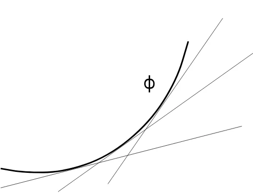
7 Jensen’s Inequality 91 7.1 Jensen’s Inequality for Conditional Expectations . . . 91
7.2 Optimal Exercise of an American Call . . . 92
7.3 Stopped Martingales . . . 94
3
8.2 is almost surely finite . . . 97
8.3 The moment generating function for . . . 99
8.4 Expectation of . . . 100
8.5 The Strong Markov Property . . . 101
8.6 General First Passage Times . . . 101
8.7 Example: Perpetual American Put . . . 102
8.8 Difference Equation . . . 106
8.9 Distribution of First Passage Times . . . 107
8.10 The Reflection Principle . . . 109
9 Pricing in terms of Market Probabilities: The Radon-Nikodym Theorem. 111 9.1 Radon-Nikodym Theorem . . . 111
9.2 Radon-Nikodym Martingales . . . 112
9.3 The State Price Density Process . . . 113
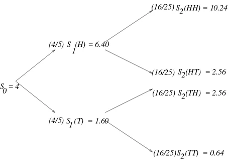
9.4 Stochastic Volatility Binomial Model . . . 116
9.5 Another Applicaton of the Radon-Nikodym Theorem . . . 118
10 Capital Asset Pricing 119 10.1 An Optimization Problem . . . 119
11 General Random Variables 123 11.1 Law of a Random Variable . . . 123
11.2 Density of a Random Variable . . . 123
11.3 Expectation . . . 124
11.4 Two random variables . . . 125
11.5 Marginal Density . . . 126
11.6 Conditional Expectation . . . 126
11.7 Conditional Density . . . 127
11.8 Multivariate Normal Distribution . . . 129
11.9 Bivariate normal distribution . . . 130
11.10MGF of jointly normal random variables . . . 130
12.2 The Stock Price Process . . . 132
12.3 Remainder of the Market . . . 133
12.4 Risk-Neutral Measure . . . 133
12.5 Risk-Neutral Pricing . . . 134
12.6 Arbitrage . . . 134
12.7 Stalking the Risk-Neutral Measure . . . 135
12.8 Pricing a European Call . . . 138
13 Brownian Motion 139 13.1 Symmetric Random Walk . . . 139
13.2 The Law of Large Numbers . . . 139
13.3 Central Limit Theorem . . . 140
13.4 Brownian Motion as a Limit of Random Walks . . . 141
13.5 Brownian Motion . . . 142
13.6 Covariance of Brownian Motion . . . 143
13.7 Finite-Dimensional Distributions of Brownian Motion . . . 144
13.8 Filtration generated by a Brownian Motion . . . 144
13.9 Martingale Property . . . 145
13.10The Limit of a Binomial Model . . . 145
13.11Starting at Points Other Than 0 . . . 147
13.12Markov Property for Brownian Motion . . . 147
13.13Transition Density . . . 149
13.14First Passage Time . . . 149
14 The Itˆo Integral 153 14.1 Brownian Motion . . . 153
14.2 First Variation . . . 153
14.3 Quadratic Variation . . . 155
14.4 Quadratic Variation as Absolute Volatility . . . 157
14.5 Construction of the It ˆo Integral . . . 158
14.6 It ˆo integral of an elementary integrand . . . 158
14.7 Properties of the It ˆo integral of an elementary process . . . 159
5
14.9 Properties of the (general) It ˆo integral . . . 163
14.10Quadratic variation of an It ˆo integral . . . 165
15 Itˆo’s Formula 167 15.1 It ˆo’s formula for one Brownian motion . . . 167
15.2 Derivation of It ˆo’s formula . . . 168
15.3 Geometric Brownian motion . . . 169
15.4 Quadratic variation of geometric Brownian motion . . . 170
15.5 Volatility of Geometric Brownian motion . . . 170
15.6 First derivation of the Black-Scholes formula . . . 170
15.7 Mean and variance of the Cox-Ingersoll-Ross process . . . 172
15.8 Multidimensional Brownian Motion . . . 173
15.9 Cross-variations of Brownian motions . . . 174
15.10Multi-dimensional It ˆo formula . . . 175
16 Markov processes and the Kolmogorov equations 177 16.1 Stochastic Differential Equations . . . 177
16.2 Markov Property . . . 178
16.3 Transition density . . . 179
16.4 The Kolmogorov Backward Equation . . . 180
16.5 Connection between stochastic calculus and KBE . . . 181
16.6 Black-Scholes . . . 183
16.7 Black-Scholes with price-dependent volatility . . . 186
17 Girsanov’s theorem and the risk-neutral measure 189 17.1 Conditional expectations underf IP . . . 191
17.2 Risk-neutral measure . . . 193
18 Martingale Representation Theorem 197 18.1 Martingale Representation Theorem . . . 197
18.2 A hedging application . . . 197
18.3 d-dimensional Girsanov Theorem . . . 199
18.4 d-dimensional Martingale Representation Theorem . . . 200
19 A two-dimensional market model 203
19.1 Hedging when,1<<1 . . . 204
19.2 Hedging when=1 . . . 205
20 Pricing Exotic Options 209 20.1 Reflection principle for Brownian motion . . . 209
20.2 Up and out European call. . . 212
20.3 A practical issue . . . 218
21 Asian Options 219 21.1 Feynman-Kac Theorem . . . 220
21.2 Constructing the hedge . . . 220
21.3 Partial average payoff Asian option . . . 221
22 Summary of Arbitrage Pricing Theory 223 22.1 Binomial model, Hedging Portfolio . . . 223
22.2 Setting up the continuous model . . . 225
22.3 Risk-neutral pricing and hedging . . . 227
22.4 Implementation of risk-neutral pricing and hedging . . . 229
23 Recognizing a Brownian Motion 233 23.1 Identifying volatility and correlation . . . 235
23.2 Reversing the process . . . 236
24 An outside barrier option 239 24.1 Computing the option value . . . 242
24.2 The PDE for the outside barrier option . . . 243
24.3 The hedge . . . 245
25 American Options 247 25.1 Preview of perpetual American put . . . 247
25.2 First passage times for Brownian motion: first method . . . 247
25.3 Drift adjustment . . . 249
25.4 Drift-adjusted Laplace transform . . . 250
7
25.6 Perpetual American put . . . 252
25.7 Value of the perpetual American put . . . 256
25.8 Hedging the put . . . 257
25.9 Perpetual American contingent claim . . . 259
25.10Perpetual American call . . . 259
25.11Put with expiration . . . 260
25.12American contingent claim with expiration . . . 261
26 Options on dividend-paying stocks 263 26.1 American option with convex payoff function . . . 263
26.2 Dividend paying stock . . . 264
26.3 Hedging at timet 1 . . . 266
27 Bonds, forward contracts and futures 267 27.1 Forward contracts . . . 269
27.2 Hedging a forward contract . . . 269
27.3 Future contracts . . . 270
27.4 Cash flow from a future contract . . . 272
27.5 Forward-future spread . . . 272
27.6 Backwardation and contango . . . 273
28 Term-structure models 275 28.1 Computing arbitrage-free bond prices: first method . . . 276
28.2 Some interest-rate dependent assets . . . 276
28.3 Terminology . . . 277
28.4 Forward rate agreement . . . 277
28.5 Recovering the interestr (t)from the forward rate . . . 278
28.6 Computing arbitrage-free bond prices: Heath-Jarrow-Morton method . . . 279
28.7 Checking for absence of arbitrage . . . 280
28.8 Implementation of the Heath-Jarrow-Morton model . . . 281
29 Gaussian processes 285 29.1 An example: Brownian Motion . . . 286
30.1 Fiddling with the formulas . . . 295
30.2 Dynamics of the bond price . . . 296
30.3 Calibration of the Hull & White model . . . 297
30.4 Option on a bond . . . 299
31 Cox-Ingersoll-Ross model 303 31.1 Equilibrium distribution ofr (t). . . 306
31.2 Kolmogorov forward equation . . . 306
31.3 Cox-Ingersoll-Ross equilibrium density . . . 309
31.4 Bond prices in the CIR model . . . 310
31.5 Option on a bond . . . 313
31.6 Deterministic time change of CIR model . . . 313
31.7 Calibration . . . 315
31.8 Tracking down' 0 (0)in the time change of the CIR model . . . 316
32 A two-factor model (Duffie & Kan) 319 32.1 Non-negativity ofY . . . 320
32.2 Zero-coupon bond prices . . . 321
32.3 Calibration . . . 323
33 Change of num´eraire 325 33.1 Bond price as num´eraire . . . 327
33.2 Stock price as num´eraire . . . 328
33.3 Merton option pricing formula . . . 329
34 Brace-Gatarek-Musiela model 335 34.1 Review of HJM under risk-neutralIP . . . 335
34.2 Brace-Gatarek-Musiela model . . . 336
34.3 LIBOR . . . 337
34.4 Forward LIBOR . . . 338
34.5 The dynamics ofL(t;) . . . 338
34.6 Implementation of BGM . . . 340
34.7 Bond prices . . . 342
9
34.9 Pricing an interest rate caplet . . . 343
34.10Pricing an interest rate cap . . . 345
34.11Calibration of BGM . . . 345
34.12Long rates . . . 346
Chapter 1
Introduction to Probability Theory
1.1
The Binomial Asset Pricing Model
Thebinomial asset pricing modelprovides a powerful tool to understand arbitrage pricing theory
and probability theory. In this course, we shall use it for both these purposes.
In the binomial asset pricing model, we model stock prices in discrete time, assuming that at each step, the stock price will change to one of two possible values. Let us begin with an initial positive stock priceS
0. There are two positive numbers,
dandu, with
0<d<u; (1.1)
such that at the next period, the stock price will be eitherdS 0 or
uS
0. Typically, we take
dandu
to satisfy0 < d < 1 < u, so change of the stock price from S 0 to
dS
0 represents a downward
movement, and change of the stock price from S 0 to
uS
0 represents an upwardmovement. It is
common to also haved= 1 u
, and this will be the case in many of our examples. However, strictly speaking, for what we are about to do we need to assume only (1.1) and (1.2) below.
Of course, stock price movements are much more complicated than indicated by the binomial asset pricing model. We consider this simple model for three reasons. First of all, within this model the concept of arbitrage pricing and its relation to risk-neutral pricing is clearly illuminated. Secondly, the model is used in practice because with a sufficient number of steps, it provides a good, compu-tationally tractable approximation to continuous-time models. Thirdly, within the binomial model we can develop the theory of conditional expectations and martingales which lies at the heart of continuous-time models.
With this third motivation in mind, we develop notation for the binomial model which is a bit different from that normally found in practice. Let us imagine that we are tossing a coin, and when we get a “Head,” the stock price moves up, but when we get a “Tail,” the price moves down. We denote the price at time1byS
1
(H)=uS
0if the toss results in head (H), and by S
1
(T)=dS 0if it
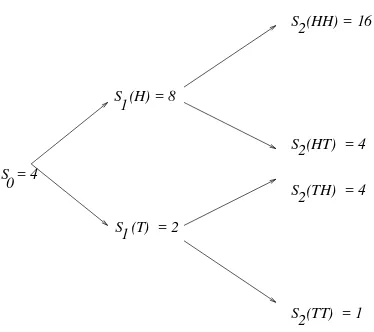
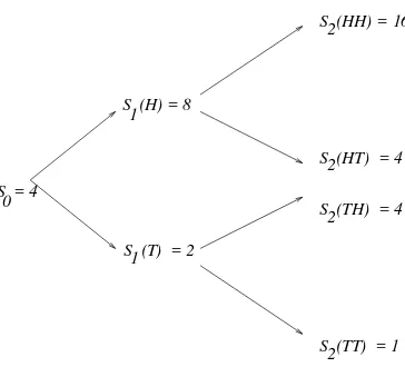
S = 4 0
S (H) = 8
S (T) = 2
S (HH) = 16
S (TT) = 1 S (HT) = 4 S (TH) = 4 1
1
2
2 2
2
Figure 1.1:Binomial tree of stock prices withS 0
=4,u=1=d=2.
results in tail (T). After the second toss, the price will be one of:
S 2
(HH)=uS 1
(H)=u 2
S 0
; S 2
(HT)=dS 1
(H)=duS 0
;
S 2
(TH)=uS 1
(T)=udS 0
; S
2
(TT)=dS 1
(T)=d 2
S 0
:
After three tosses, there are eight possible coin sequences, although not all of them result in different stock prices at time3.
For the moment, let us assume that the third toss is the last one and denote by
=fHHH ;HHT;HTH ;HTT;THH ;THT;TTH ;TTTg
the set of all possible outcomes of the three tosses. The setof all possible outcomes of a
ran-dom experiment is called thesample spacefor the experiment, and the elements! ofare called
sample points. In this case, each sample point! is a sequence of length three. We denote thek-th
component of!by!
k. For example, when
! =HTH, we have! 1
=H,! 2
=T and! 3
=H.
The stock priceS
k at time
kdepends on the coin tosses. To emphasize this, we often writeS k
(!).
Actually, this notation does not quite tell the whole story, for whileS
3 depends on all of !, S
2
depends on only the first two components of!,S
1 depends on only the first component of !, and S
0does not depend on
!at all. Sometimes we will use notation suchS 2
(! 1
;! 2
)just to record more
explicitly howS
2depends on
!=(! 1
;! 2
;! 3
).
Example 1.1 SetS 0
=4,u = 2andd = 1 2
. We have then the binomial “tree” of possible stock prices shown in Fig. 1.1. Each sample point! = (!
1 ;!
2 ;!
3
)represents a path through the tree.
Thus, we can think of the sample spaceas either the set of all possible outcomes from three coin
tosses or as the set of all possible paths through the tree.
To complete our binomial asset pricing model, we introduce amoney marketwithinterest rater;
CHAPTER 1. Introduction to Probability Theory 13
rate for bothborrowingandlending. (This is not as ridiculous as it first seems, because in a many applications of the model, an agent is either borrowing or lending (not both) and knows in advance which she will be doing; in such an application, she should takerto be the rate of interest for her
activity.) We assume that
d<
1 +
r<u: (1.2)The model would not make sense if we did not have this condition. For example, if
1+
ru, thenthe rate of return on the money market is always at least as great as and sometimes greater than the return on the stock, and no one would invest in the stock. The inequalityd
1 +
rcannot happenunless eitherris negative (which never happens, except maybe once upon a time in Switzerland) or d
1
. In the latter case, the stock does not really go “down” if we get a tail; it just goes up lessthan if we had gotten a head. One should borrow money at interest raterand invest in the stock,
since even in the worst case, the stock price rises at least as fast as the debt used to buy it.
With the stock as the underlying asset, let us consider a European call option with strike price
K>
0
and expiration time1
. This option confers the right to buy the stock at time1
forKdollars,and so is worthS 1
,Kat time
1
ifS 1,Kis positive and is otherwise worth zero. We denote by V
1
(
!
) = (
S1
(
!
)
,K)
+
= max
fS1
(
!
)
,K ;0
gthe value (payoff) of this option at expiration. Of course,V 1
(
!
)
actually depends only on! 1, andwe can and do sometimes writeV 1
(
!
1
)
rather than V1
(
!
)
. Our first task is to compute thearbitragepriceof this option at time zero.
Suppose at time zero you sell the call forV
0 dollars, where V
0is still to be determined. You now
have an obligation to pay off
(
uS 0,K
)
+if! 1
=
H and to pay off
(
dS 0,K
)
+if! 1
=
T. At
the time you sell the option, you don’t yet know which value!
1 will take. Youhedgeyour short
position in the option by buying
0shares of stock, where0is still to be determined. You can usethe proceedsV
0of the sale of the option for this purpose, and then borrow if necessary at interest
raterto complete the purchase. If V
0 is more than necessary to buy the
0 shares of stock, youinvest the residual money at interest rater. In either case, you will haveV 0
,
0 S
0dollars invested
in the money market, where this quantity might be negative. You will also own
0shares of stock.If the stock goes up, the value of your portfolio (excluding the short position in the option) is
0S 1
(
H
) + (1 +
r)(
V0
,
0 S
0
)
;and you need to haveV 1
(
H
)
. Thus, you want to chooseV0and
0so that V1
(
H
) =
0S 1
(
H
) + (1 +
r)(
V0
,
0 S
0
)
: (1.3)
If the stock goes down, the value of your portfolio is
0S 1
(
T
) + (1 +
r)(
V0
,
0 S
0
)
;and you need to haveV 1
(
T
)
. Thus, you want to chooseV0and
0to also have V1
(
T
) =
0S 1
(
T
) + (1 +
r)(
V0
,
0 S
0
)
These are two equations in two unknowns, and we solve them below
Subtracting (1.4) from (1.3), we obtain
V 1
(H),V 1
(T)= 0
(S 1
(H),S 1
(T)); (1.5)
so that
0
= V
1
(H),V 1
(T) S
1
(H),S 1
(T)
: (1.6)
This is a discrete-time version of the famous “delta-hedging” formula for derivative securities, ac-cording to which the number of shares of an underlying asset a hedge should hold is the derivative (in the sense of calculus) of the value of the derivative security with respect to the price of the underlying asset. This formula is so pervasive the when a practitioner says “delta”, she means the derivative (in the sense of calculus) just described. Note, however, that mydefinitionof
0 is the
number of shares of stock one holds at time zero, and (1.6) is a consequence of this definition, not the definition of
0 itself. Depending on how uncertainty enters the model, there can be cases
in which the number of shares of stock a hedge should hold is not the (calculus) derivative of the derivative security with respect to the price of the underlying asset.
To complete the solution of (1.3) and (1.4), we substitute (1.6) into either (1.3) or (1.4) and solve forV
0. After some simplification, this leads to the formula
V 0
= 1 1+r
1+r,d u,d
V 1
(H)+
u,(1+r ) u,d
V 1
(T)
: (1.7)
This is thearbitrage pricefor the European call option with payoffV
1 at time
1. To simplify this
formula, we define
~ p
=
1+r,d u,d
; q~ =
u,(1+r ) u,d
=1,p;~ (1.8)
so that (1.7) becomes
V 0
= 1 1+r
[~pV 1
(H)+qV~ 1
(T)]: (1.9)
Because we have takend < u, bothp~andq~are defined,i.e., the denominator in (1.8) is not zero.
Because of (1.2), bothp~andq~are in the interval(0;1), and because they sum to1, we can regard
them as probabilities ofH andT, respectively. They are therisk-neutralprobabilites. They
ap-peared when we solved the two equations (1.3) and (1.4), and have nothing to do with the actual probabilities of gettingHorT on the coin tosses. In fact, at this point, they are nothing more than
a convenient tool for writing (1.7) as (1.9).
We now consider a European call which pays offKdollars at time2. At expiration, the payoff of
this option isV 2
=(S
2 ,K)
+
, whereV 2 and
S
2 depend on !
1 and !
2, the first and second coin
tosses. We want to determine the arbitrage price for this option at time zero. Suppose an agent sells the option at time zero forV
0 dollars, where V
0is still to be determined. She then buys
CHAPTER 1. Introduction to Probability Theory 15
of stock, investingV 0
,
0 S
0dollars in the money market to finance this. At time
1, the agent has
a portfolio (excluding the short position in the option) valued at
X
Although we do not indicate it in the notation,S
1 and therefore X
1 depend on !
1, the outcome of
the first coin toss. Thus, there are really two equations implicit in (1.10):
X
After the first coin toss, the agent hasX
1dollars and can readjust her hedge. Suppose she decides to
now hold
1 shares of stock, where
1 is allowed to depend on !
1 because the agent knows what
value!
1 has taken. She invests the remainder of her wealth, X
1
,
1 S
1 in the money market. In
the next period, her wealth will be given by the right-hand side of the following equation, and she wants it to beV
2. Therefore, she wants to have V
Although we do not indicate it in the notation,S 2and
V
2depend on !
1and !
2, the outcomes of the
first two coin tosses. Considering all four possible outcomes, we can write (1.11) as four equations:
V
We now have six equations, the two represented by (1.10) and the four represented by (1.11), in the six unknownsV
0,
To solve these equations, and thereby determine the arbitrage priceV
0at time zero of the option and
the hedging portfolio 0,
Subtracting one of these from the other and solving for 1
(T), we obtain the “delta-hedging
for-mula”
and substituting this into either equation, we can solve for
Equation (1.13), gives the value the hedging portfolio should have at time1if the stock goes down
between times0and1. We define this quantity to be thearbitrage value of the option at time1if !
The hedger should choose her portfolio so that her wealth X 1
defined by (1.14). This formula is analgous to formula (1.9), but postponed by one step. The first two equations implicit in (1.11) lead in a similar way to the formulas
This is again analgous to formula (1.9), postponed by one step. Finally, we plug the valuesX 1
(T) into the two equations implicit in (1.10). The solution of these
equa-tions for 0 and
V
0 is the same as the solution of (1.3) and (1.4), and results again in (1.6) and
(1.9).
The pattern emerging here persists, regardless of the number of periods. IfV
k denotes the value at
timekof a derivative security, and this depends on the firstkcoin tosses! 1
k ,1 are known, the portfolio to hedge a short position
should hold k ,1
(! 1
;:::;! k ,1
)shares of stock, where
and the value at timek,1of the derivative security, when the firstk,1coin tosses result in the
outcomes! 1
1.2
Finite Probability Spaces
Letbe a set with finitely many elements. An example to keep in mind is
=fHHH ;HHT;HTH ;HTT;THH ;THT;TTH ;TTTg (2.1)
of all possible outcomes of three coin tosses. LetF be the set of all subsets of. Some sets inF
CHAPTER 1. Introduction to Probability Theory 17
Definition 1.1 A probability measureIP is a function mapping F into[0;1] with the following
properties:
Probability measures have the following interpretation. LetAbe a subset ofF. Imagine thatis
the set of all possible outcomes of some random experiment. There is a certain probability, between
0 and1, that when that experiment is performed, the outcome will lie in the set A. We think of IP(A)as this probability.
Example 1.2 Suppose a coin has probability1 3
forHand 2 3
forT. For the individual elements of in (2.1), define
For example,
IPfHHH ;HHT;HTH ;HTTg=
which is another way of saying that the probability ofHon the first toss is 1 3
.
As in the above example, it is generally the case that we specify a probability measure on only some of the subsets ofand then use property (ii) of Definition 1.1 to determineIP(A)for the remaining
setsA2F. In the above example, we specified the probability measure only for the sets containing
a single element, and then used Definition 1.1(ii) in the form (2.2) (see Problem 1.4(ii)) to determine
IP for all the other sets inF.
Definition 1.2 Let be a nonempty set. A-algebra is a collection G of subsets ofwith the
following three properties:
(ii) IfA2G, then its complementA c
2G,
(iii) IfA 1
;A 2
;A 3
;::: is a sequence of sets inG, then[ 1 k =1
A
k is also in G.
Here are some important-algebras of subsets of the setin Example 1.2:
F 0
= (
;; )
;
F 1
= (
;;;fHHH ;HHT;HTH ;HTTg;fTHH ;THT;TTH ;TTTg )
;
F 2
= (
;;;fHHH ;HHTg;fHTH ;HTTg;fTHH ;THTg;fTTH ;TTTg;
and all sets which can be built by taking unions of these
) ; F
3
= F =The set of all subsets of:
To simplify notation a bit, let us define
A H
=fHHH ;HHT;HTH ;HTTg=fHon the first tossg; A
T
=fTHH ;THT;TTH ;TTTg=fT on the first tossg;
so that
F 1
=f;;;A H
;A T
g;
and let us define
A HH
=fHHH ;HHTg=fHHon the first two tossesg; A
HT
=fHTH ;HTTg=fHT on the first two tossesg; A
TH
=fTHH ;THTg=fTHon the first two tossesg; A
TT
=fTTH ;TTTg=fTT on the first two tossesg;
so that
F 2
= f;;;A HH
;A HT
;A TH
;A TT
; A
H ;A
T ;A
HH [A
TH ;A
HH [A
TT ;A
HT [A
TH ;A
HT [A
TT ; A
c HH
;A c HT
;A c TH
;A c TT
g:
We interpret-algebras as a record of information. Suppose the coin is tossed three times, and you
are not told the outcome, but you are told, for every set inF
1whether or not the outcome is in that
set. For example, you would be told that the outcome is not in;and is in. Moreover, you might
be told that the outcome is not inA
H but is in A
T. In effect, you have been told that the first toss
was aT, and nothing more. The-algebraF
1is said to contain the “information of the first toss”,
which is usually called the “information up to time1”. Similarly,F
CHAPTER 1. Introduction to Probability Theory 19
the first two tosses,” which is the “information up to time2.” The-algebraF 3
=F contains “full
information” about the outcome of all three tosses. The so-called “trivial”-algebraF
0contains no
information. Knowing whether the outcome!of the three tosses is in;(it is not) and whether it is
in(it is) tells you nothing about!
Definition 1.3 Letbe a nonempty finite set. Afiltrationis a sequence of-algebrasF 0
;F 1
;F 2
;:::;F n
such that each-algebra in the sequence contains all the sets contained by the previous-algebra.
Definition 1.4 Letbe a nonempty finite set and letF be the-algebra of all subsets of. A
random variable is a function mappingintoIR.
Example 1.3 Letbe given by (2.1) and consider the binomial asset pricing Example 1.1, where S
0
= 4, u = 2 and d = 1 2
. Then S 0,
S 1,
S 2 and
S
3 are all random variables. For example, S
2
(HHT)=u 2
S 0
=16. The “random variable”S
0 is really not random, since S
0
(!)=4for all ! 2 . Nonetheless, it is a function mappingintoIR, and thus technically a random variable,
albeit a degenerate one.
A random variable mapsintoIR, and we can look at the preimage under the random variable of
sets inIR. Consider, for example, the random variableS
2of Example 1.1. We have S
2
(HHH)=S
2
(HHT)=16; S
2
(HTH)=S 2
(HTT)=S 2
(THH)=S 2
(THT)=4; S
2
(TTH)=S 2
(TTT)=1:
Let us consider the interval[4;27]. The preimage underS
2of this interval is defined to be f!2;S
2
(!)2[4;27]g=f! 2;4S 2
27g=A c TT
:
The complete list of subsets ofwe can get as preimages of sets inIRis:
;;;A HH
;A HT
[A TH
;A TT
;
and sets which can be built by taking unions of these. This collection of sets is a-algebra, called
the -algebra generated by the random variableS
2, and is denoted by (S
2
). The information
content of this -algebra is exactly the information learned by observing S
2. More specifically,
suppose the coin is tossed three times and you do not know the outcome!, but someone is willing
to tell you, for each set in(S 2
), whether! is in the set. You might be told, for example, that!is
not inA
HH, is in A
HT [A
TH, and is not in A
TT. Then you know that in the first two tosses, there
was a head and a tail, and you know nothing more. This information is the same you would have gotten by being told that the value ofS
2
(!)is4.
Note thatF
2 defined earlier contains all the sets which are in (S
2
), and even more. This means
that the information in the first two tosses is greater than the information inS
2. In particular, if you
see the first two tosses, you can distinguishA
HT from A
TH, but you cannot make this distinction
from knowing the value ofS
Definition 1.5 Letbe a nonemtpy finite set and letF be the-algebra of all subsets of. LetX
be a random variable on(;F). The-algebra(X)generated byXis defined to be the collection
of all sets of the formf! 2;X(!)2Ag, whereAis a subset ofIR. LetGbe a sub--algebra of F. We say thatXisG-measurableif every set in(X)is also inG.
Note: We normally write simplyfX 2Agrather thanf!2;X(!)2Ag.
Definition 1.6 Letbe a nonempty, finite set, letFbe the-algebra of all subsets of, letIP be
a probabilty measure on(;F), and letX be a random variable on. Given any setA IR, we
define theinduced measureofAto be
L X
(A)
=IPfX 2Ag:
In other words, the induced measure of a setAtells us the probability thatXtakes a value inA. In
the case ofS
2above with the probability measure of Example 1.2, some sets in
IRand their induced
measures are:
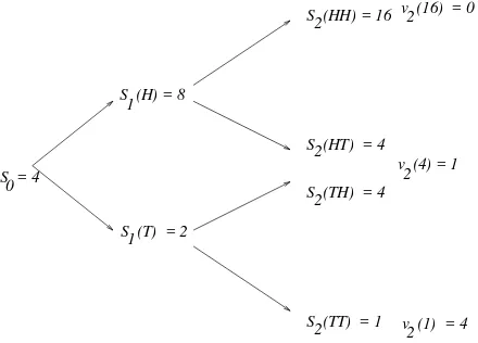
L S2
(;)=IP(;)=0; L
S 2
(IR)=IP()=1; L
S 2
[0;1)=IP()=1; L
S 2
[0;3]=IPfS 2
=1g=IP(A TT
)=
2 3
2
:
In fact, the induced measure ofS
2 places a mass of size
1 3
2 =
1 9
at the number16, a mass of size 4
9
at the number4, and a mass of size
2 3
2 =
4 9
at the number1. A common way to record this
information is to give thecumulative distribution functionF S2
(x)ofS
2, defined by
F S
2 (x)
=IP(S
2
x)=
8 > > > < > > > :
0; ifx<1; 4
9
; if1x<4; 8
9
; if4x<16; 1; if16x:
(2.3)
By the distributionof a random variable X, we mean any of the several ways of characterizing L
X. If
X is discrete, as in the case ofS
2 above, we can either tell where the masses are and how
large they are, or tell what the cumulative distribution function is. (Later we will consider random variablesXwhich have densities, in which case the induced measure of a setAIRis the integral
of the density over the setA.)
Important Note. In order to work through the concept of a risk-neutral measure, we set up the definitions to make a clear distinction between random variables and their distributions.
Arandom variableis a mapping fromtoIR, nothing more. It has an existence quite apart from
discussion of probabilities. For example, in the discussion above, S 2
(TTH) = S 2
(TTT) = 1,
regardless of whether the probability forHis 1 3
or 1 2
CHAPTER 1. Introduction to Probability Theory 21
Thedistributionof a random variable is a measureL
X on
IR, i.e., a way of assigning probabilities
to sets inIR. It depends on the random variableXand the probability measureIP we use in. If we
set the probability ofHto be 1 3
, thenL S
2 assigns mass 1 9
to the number16. If we set the probability
ofH to be 1 2
, thenL S
2 assigns mass 1 4
to the number16. The distribution ofS
2has changed, but
the random variable has not. It is still defined by
S
Thus, a random variable can have more than one distribution (a “market” or “objective” distribution, and a “risk-neutral” distribution).
In a similar vein, twodifferent random variablescan have thesame distribution. Suppose in the binomial model of Example 1.1, the probability ofH and the probability ofT is
1 2
. Consider a European call with strike price14expiring at time2. The payoff of the call at time2is the random
variable(S 2
,14) +
, which takes the value2if!=HHHor!=HHT, and takes the value0in
every other case. The probability the payoff is2is 1 4
, and the probability it is zero is3 4
. Consider also a European put with strike price3expiring at time2. The payoff of the put at time2is(3,S
put is2with probability 1 4
and0with probability 3 4
. The payoffs of the call and the put are different random variables having the same distribution.
Definition 1.7 Letbe a nonempty, finite set, letFbe the-algebra of all subsets of, letIP be
a probabilty measure on(;F), and letXbe a random variable on. Theexpected valueofXis
defined to be
IEX
Notice that the expected value in (2.4) is defined to be a sumover the sample space. Sinceis a
finite set,Xcan take only finitely many values, which we labelx 1
;:::;x
n. We can partition into
Thus, although the expected value is defined as a sum over the sample space, we can also write it
as a sum overIR.
To make the above set of equations absolutely clear, we considerS
2 with the distribution given by
(2.3). The definition ofIES 2is IES
2
= S
2
(HHH)IPfHHHg+S 2
(HHT)IPfHHTg +S
2
(HTH)IPfHTHg+S 2
(HTT)IPfHTTg +S
2
(THH)IPfTHHg+S 2
(THT)IPfTHTg +S
2
(TTH)IPfTTHg+S 2
(TTT)IPfTTTg = 16IP(A
HH
)+4IP(A HT
[A TH
)+1IP(A TT
) = 16IPfS
2
=16g+4IPfS 2
=4g+1IPfS 2
=1g
= 16L
S2
f16g+4L S2
f4g+1L S2
f1g
= 16
1 9
+4 4 9
+4 4 9 =
48 9
:
Definition 1.8 Letbe a nonempty, finite set, letFbe the-algebra of all subsets of, letIP be a
probabilty measure on(;F), and letXbe a random variable on. ThevarianceofXis defined
to be the expected value of(X,IEX) 2
, i.e.,
Var(X) =
X ! 2
(X(!),IEX) 2
IPf!g: (2.5)
One again, we can rewrite (2.5) as a sum overIRrather than over. Indeed, ifXtakes the values x
1 ;:::;x
n, then
Var(X)= n X k =1
(x k
,IEX) 2
IPfX =x k
g= n X k =1
(x k
,IEX) 2
L X
(x k
):
1.3
Lebesgue Measure and the Lebesgue Integral
In this section, we consider the set of real numbersIR, which is uncountably infinite. We define the
Lebesgue measureof intervals inIRto be their length. This definition and the properties of measure
determine the Lebesgue measure of many, but not all, subsets ofIR. The collection of subsets of IRwe consider, and for which Lebesgue measure is defined, is the collection ofBorel setsdefined
below.
We use Lebesgue measure to construct the Lebesgue integral, a generalization of the Riemann integral. We need this integral because, unlike the Riemann integral, it can be defined on abstract spaces, such as the space of infinite sequences of coin tosses or the space of paths of Brownian motion. This section concerns the Lebesgue integral on the space IRonly; the generalization to
CHAPTER 1. Introduction to Probability Theory 23
Definition 1.9 TheBorel-algebra, denotedB (IR), is the smallest-algebra containing all open
intervals inIR. The sets inB (IR)are calledBorel sets.
Every set which can be written down and just about every set imaginable is inB (IR). The following
discussion of this fact uses the-algebra properties developed in Problem 1.3.
By definition, every open interval(a;b)is inB (IR), whereaandbare real numbers. SinceB (IR)is
a-algebra, every union of open intervals is also inB (IR). For example, for every real numbera,
theopen half-line
(a;1)= 1 [ n=1
(a;a+n)
is a Borel set, as is
(,1;a)= 1 [ n=1
(a,n;a):
For real numbersaandb, the union
(,1;a)[(b;1)
is Borel. SinceB (IR)is a-algebra, every complement of a Borel set is Borel, soB (IR)contains
[a;b]=
(,1;a)[(b;1)
c :
This shows that every closed interval is Borel. In addition, theclosed half-lines
[a;1)= 1 [ n=1
[a;a+n]
and
(,1;a]= 1 [ n=1
[a,n;a]
are Borel. Half-open and half-closed intervals are also Borel, since they can be written as intersec-tions of open half-lines and closed half-lines. For example,
(a;b]=(,1;b]\(a;1):
Every set which contains only one real number is Borel. Indeed, ifais a real number, then
fag= 1 \ n=1
a,
1 n
;a+ 1 n
:
This means that every set containing finitely many real numbers is Borel; ifA =fa 1
;a 2
;:::;a n
g,
then
A= n [ k =1
fa k
In fact, every set containing countably infinitely many numbers is Borel; ifA=fa
This means that the set of rational numbers is Borel, as is its complement, the set of irrational numbers.
There are, however, sets which are not Borel. We have just seen that any non-Borel set must have uncountably many points.
Example 1.4 (The Cantor set.) This example gives a hint of how complicated a Borel set can be. We use it later when we discuss the sample space for an infinite sequence of coin tosses.
Consider the unit interval[0;1], and remove the middle half, i.e., remove the open interval
A
The remaining set
C
has two pieces. From each of these pieces, remove the middle half, i.e., remove the open set
A
The remaining set
C
has four pieces. Continue this process, so at stagek, the setC
k has 2
k
pieces, and each piece has
length 1
4
is defined to be the set of points not removed at any stage of this nonterminating process.
Note that the length ofA
1, the first set removed, is
1 2
. The “length” ofA
2, the second set removed,
is 1
, and in general, the length of the
k-th set removed is2
,k
. Thus, the total length removed is
1
and so the Cantor set, the set of points not removed, has zero “length.”
Despite the fact that the Cantor set has no “length,” there are lots of points in this set. In particular,
none of the endpoints of the pieces of the setsC
1
are all inC. This is a countably infinite set of points. We shall see eventually that the Cantor set
CHAPTER 1. Introduction to Probability Theory 25
Definition 1.10 LetB
(
IR)
be the-algebra of Borel subsets ofIR. Ameasure on(
IR;B(
IR))
is afunctionmappingBinto
[0
;1]
with the following properties:(i)
(
;) = 0
,(ii) IfA 1
;A 2
;:::is a sequence of disjoint sets inB
(
IR)
, then1 [ k =1
A k
!
=
1X k =1
(
A k)
:
Lebesgue measureis defined to be the measure on
(
IR;B(
IR))
which assigns the measure of eachinterval to be its length. Following Williams’s book, we denote Lebesgue measure by 0.
A measure has all the properties of a probability measure given in Problem 1.4, except that the total measure of the space is not necessarily
1
(in fact,0
(
IR
) =
1), one no longer has the equation(
Ac
) = 1
,
(
A)
in Problem 1.4(iii), and property (v) in Problem 1.4 needs to be modified to say:
(v) IfA 1
;A 2
;:::is a sequence of sets inB
(
IR)
withA 1A
2
and
(
A 1)
<1, then
1 \ k =1
A k
!
= lim
n!1(
A n)
:
To see that the additional requirment
(
A 1)
<1is needed in (v), consider A
1
= [1
;1)
;A2
= [2
;1)
;A3
= [3
;1
)
;::::Then\ 1 k =1
A k
=
;, so 0
(
\ 1 k =1
A
k
) = 0
, butlim
n!10
(
A n
) =
1.
We specify that the Lebesgue measure of each interval is its length, and that determines the Lebesgue measure of all other Borel sets. For example, the Lebesgue measure of the Cantor set in Example 1.4 must be zero, because of the “length” computation given at the end of that example.
The Lebesgue measure of a set containing only one point must be zero. In fact, since
fag
a,
1
n ;a
+ 1
n
for every positive integern, we must have
0
0
fag
0
a,
1
n ;a
+ 1
n
= 2
n :
Lettingn!1, we obtain
0
The Lebesgue measure of a set containing countably many points must also be zero. Indeed, if
A=fa 1
;a 2
;:::g, then
0
(A)= 1 X k =1
0
fa k
g= 1 X k =1
0=0:
The Lebesgue measure of a set containing uncountably many points can be either zero, positive and finite, or infinite. We may not compute the Lebesgue measure of an uncountable set by adding up the Lebesgue measure of its individual members, because there is no way to add up uncountably many numbers. The integral was invented to get around this problem.
In order to think about Lebesgue integrals, we must first consider the functions to be integrated.
Definition 1.11 Letf be a function from IRtoIR. We say thatf isBorel-measurableif the set fx2 IR;f(x) 2 Agis inB (IR)wheneverA 2B (IR). In the language of Section 2, we want the
-algebra generated byfto be contained inB (IR).
Definition 3.4 is purely technical and has nothing to do with keeping track of information. It is difficult to conceive of a function which is not Borel-measurable, and we shall pretend such func-tions don’t exist. Hencefore, “function mappingIRtoIR” will mean “Borel-measurable function
mappingIRtoIR” and “subset ofIR” will mean “Borel subset ofIR”.
Definition 1.12 Anindicator functiongfromIRtoIRis a function which takes only the values0
and1. We call
A
=fx2IR;g(x)=1g
the setindicatedbyg. We define theLebesgue integralofgto be Z
IR gd
0
=
0 (A):
Asimple functionhfromIRtoIRis a linear combination of indicators, i.e., a function of the form
h(x)= n X k =1 c
k g
k (x);
where eachg
k is of the form
g k
(x)= (
1; ifx2A k
; 0; ifx2=A
k ;
and eachc
k is a real number. We define theLebesgue integralof hto be Z
R hd
0 =
n X k =1 c
k Z
IR g
k d
0 =
n X k =1 c
k
0 (A
k ):
Letf be a nonnegative function defined on IR, possibly taking the value1 at some points. We
define theLebesgue integraloff to be Z
IR fd
0 =sup
Z IR
hd 0
;his simple andh(x)f(x)for everyx2IR
CHAPTER 1. Introduction to Probability Theory 27
It is possible that this integral is infinite. If it is finite, we say thatf is integrable.
Finally, letf be a function defined onIR, possibly taking the value1at some points and the value ,1at other points. We define thepositiveandnegative partsoff to be
f
respectively, and we define theLebesgue integraloff to be Z
provided the right-hand side is not of the form1,1. If both R
0are finite
(or equivalently,
R
Letf be a function defined onIR, possibly taking the value1at some points and the value,1at
other points. LetAbe a subset ofIR. We define
is theindicator function ofA.
The Lebesgue integral just defined is related to the Riemann integral in one very important way: if the Riemann integral
R b a
f
(
x)
dxis defined, then the Lebesgue integral R[a;b]
fd
0 agrees with the
Riemann integral. The Lebesgue integral has two important advantages over the Riemann integral. The first is that the Lebesgue integral is defined for more functions, as we show in the following examples.
Example 1.5 LetQbe the set of rational numbers in
[0
;1]
, and considerf=
lIQ. Being a countable
set,Qhas Lebesgue measure zero, and so the Lebesgue integral off over
[0
;1]
is Z[0;1]
fd
0
= 0
:To compute the Riemann integral
R
;
1]
into subintervals[
x 0subinterval
[
x k ,1;x
k
]
there is a rational point qk, where f
(
qk
) = 1
, and there is also an irrationalpointr
k, where f
(
rk
) = 0
. We approximate the Riemann integral from above by theupper sumn
and we also approximate it from below by thelower sum
No matter how fine we take the partition of[0;1], the upper sum is always1and the lower sum is
always0. Since these two do not converge to a common value as the partition becomes finer, the
Riemann integral is not defined.
Example 1.6 Consider the function
f(x) =
(
1; ifx=0; 0; ifx6=0:
This is not a simple function because simple function cannot take the value1. Every simple
function which lies between0andf is of the form
h(x) =
(
y; ifx=0; 0; ifx6=0;
for somey2[0;1), and thus has Lebesgue integral Z
IR hd
0
=y
0
f0g=0:
It follows that
Z IR
fd 0
=sup Z
IR hd
0
;his simple andh(x)f(x)for everyx2IR
=0:
Now consider the Riemann integral
R 1 ,1
f(x)dx, which for this function f is the same as the
Riemann integral
R 1 ,1
f(x)dx. When we partition[,1;1]into subintervals, one of these will contain
the point0, and when we compute the upper approximating sum for R
1 ,1
f(x)dx, this point will
contribute1times the length of the subinterval containing it. Thus the upper approximating sum is 1. On the other hand, the lower approximating sum is0, and again the Riemann integral does not
exist.
The Lebesgue integral has alllinearityandcomparisonproperties one would expect of an integral. In particular, for any two functionsf andgand any real constantc,
Z IR
(f +g)d 0
= Z
IR fd
0 +
Z IR
gd 0
; Z
IR cfd
0
= c
Z IR
fd
0 ;
and wheneverf(x)g(x)for allx2IR, we have Z
IR
fd
0
Z IR
gdd 0
:
Finally, ifAandBare disjoint sets, then Z
A[B
fd
0 =
Z A
fd
0 +
Z B
fd
CHAPTER 1. Introduction to Probability Theory 29
There are threeconvergence theoremssatisfied by the Lebesgue integral. In each of these the sit-uation is that there is a sequence of functionsf
n
;n
= 1
;2
;::: convergingpointwiseto a limitingfunctionf.Pointwise convergencejust means that
lim
n!1 f
n
(
x
) =
f(
x)
for everyx2IR:There are no such theorems for the Riemann integral, because the Riemann integral of the limit-ing functionf is too often not defined. Before we state the theorems, we given two examples of
pointwise convergence which arise in probability theory.
Example 1.7 Consider a sequence of normal densities, each with variance
1
and then-th havingmeann:
These converge pointwise to the function
f
(
x) = 0
for everyx2IR:We have
R
Example 1.8 Consider a sequence of normal densities, each with mean
0
and then-th havingvari-ance 1
These converge pointwise to the function
f
(
x)
We have again
R
functionf is not the Dirac delta; the Lebesgue integral of this function was already seen in Example
1.6 to be zero.
Theorem 3.1 (Fatou’s Lemma)Letf n
;n
= 1
;2
;::: be a sequence of nonnegative functionscon-verging pointwise to a functionf. Then
Z IR
fd 0
liminf
n!1
0is defined, then Fatou’s Lemma has the simpler conclusion Z
This is the case in Examples 1.7 and 1.8, where
whileR IR
fd
0
= 0
. We could modify either Example 1.7 or 1.8 by setting gn
=
fn if
nis even,
butg n
= 2
f nif
nis odd. Now R
IR g
n d
0
= 1
ifnis even, but R
IR g
n d
0
= 2
ifnis odd. The
sequence f R
IR g
n d
0 g
1 n=1
has two cluster points,
1
and2
. By definition, the smaller one,1
, isliminf
n!1R IR
g n
d
0and the larger one,
2
, islimsup
n!1R IR
g n
d
0. Fatou’s Lemma guarantees
that even the smaller cluster point will be greater than or equal to the integral of the limiting function. The key assumption in Fatou’s Lemma is that all the functions take only nonnegative values. Fatou’s Lemma does not assume much but it is is not very satisfying because it does not conclude that
Z IR
fd
0
= lim
n!1 Z
IR f
n d
0 :
There are two sets of assumptions which permit this stronger conclusion.
Theorem 3.2 (Monotone Convergence Theorem)Letf n
;n
= 1
;2
;::: be a sequence of functionsconverging pointwise to a functionf. Assume that
0
f1
(
x)
f2
(
x)
f3
(
x
)
for everyx2IR:Then Z
IR fd
0
= lim
n!1 Z
IR f
n d
0 ;
where both sides are allowed to be1.
Theorem 3.3 (Dominated Convergence Theorem)Letf n
;n
= 1
;2
;:::be a sequence of functions,which may take either positive or negative values, converging pointwise to a functionf. Assume
that there is a nonnegative integrable functiong(i.e.,
R IR
gd 0
<1) such that
jf n
(
x
)
jg(
x)
for everyx2IRfor everyn:Then Z
IR fd
0
= lim
n!1 Z
IR f
n d
0 ;
and both sides will be finite.
1.4
General Probability Spaces
Definition 1.13 Aprobability space
(
;F;IP)
consists of three objects:(i)
, a nonempty set, called the sample space, which contains all possible outcomes of some random experiment;(ii) F, a-algebra of subsets of
;(iii) IP, a probability measure on
(
;F)
, i.e., a function which assigns to each setA2Fa number IP(
A)
2[0
;1]
, which represents the probability that the outcome of the random experimentCHAPTER 1. Introduction to Probability Theory 31
Remark 1.1 We recall from Homework Problem 1.4 that a probability measureIP has the following
properties:
(a) IP
(
;) = 0
.(b) (Countable additivity) IfA 1
;A 2
;:::is a sequence of disjoint sets inF, then
IP 1 [
k
=1 Ak
!
=
1X
k
=1IP
(
Ak
)
:(c) (Finite additivity) Ifnis a positive integer andA 1
;:::;A
n
are disjoint sets inF, then IP(
A1
[[A
n
) =
IP(
A 1) +
+
IP(
An
)
:(d) IfAandBare sets inF andAB, then
IP
(
B) =
IP(
A) +
IP(
BnA)
:In particular,
IP
(
B)
IP(
A)
:(d) (Continuity from below.) IfA 1
;A 2
;::: is a sequence of sets inFwithA 1
A
2
, then
IP 1 [
k
=1 Ak
!
= lim
n
!1
IP
(
An
)
:(d) (Continuity from above.) IfA 1
;A 2
;::: is a sequence of sets inFwithA 1
A
2
, then
IP 1 \
k
=1 Ak
!
= lim
n
!1
IP
(
An
)
:We have already seen some examples of finite probability spaces. We repeat these and give some examples of infinite probability spaces as well.
Example 1.9 Finite coin toss space.
Toss a coinntimes, so that
is the set of all sequences of H andT which have ncomponents.We will use this space quite a bit, and so give it a name:
n
. LetF be the collection of all subsetsof
n
. Suppose the probability ofH on each toss isp, a number between zero and one. Then theprobability ofTisq
= 1
,p. For each!= (
! 1;! 2
;:::;!
n
)
inn
, we define IPf!g
=
pNumber of H in !
qNumber of T in !
:For eachA2F, we define
IP
(
A)
=
X!
2A
IPf!g: (4.1)
We can defineIP
(
A)
this way becauseAhas only finitely many elements, and so only finitely manyExample 1.10 Infinite coin toss space.
Toss a coin repeatedly without stopping, so thatis the set of all nonterminating sequences ofH
andT. We call this space
1. This is an uncountably infinite space, and we need to exercise some
care in the construction of the-algebra we will use here.
For each positive integern, we defineF
nto be the
-algebra determined by the firstntosses. For
example,F
2contains four basic sets, A
HH
= f! =(!
1 ;!
2 ;!
3
;:::);! 1
=H ;! 2
=Hg = The set of all sequences which begin withHH ; A
HT
= f! =(!
1 ;!
2 ;!
3
;:::);! 1
=H ;! 2
=Tg = The set of all sequences which begin withHT; A
TH
= f! =(!
1 ;!
2 ;!
3
;:::);! 1
=T;! 2
=Hg = The set of all sequences which begin withTH ; A
TT
= f! =(!
1 ;!
2 ;!
3
;:::);! 1
=T;! 2
=Tg = The set of all sequences which begin withTT:
BecauseF 2 is a
-algebra, we must also put into it the sets;,, and all unions of the four basic
sets.
In the -algebra F, we put every set in every -algebra F
n, where
n ranges over the positive
integers. We also put in every other set which is required to makeF be a-algebra. For example,
the set containing the single sequence
fHHHHHg=fHon every tossg
is not in any of theF n
-algebras, because it depends on all the components of the sequence and
not just the firstncomponents. However, for each positive integern, the set
fHon the firstntossesg
is inF
nand hence in
F. Therefore,
fHon every tossg= 1 \ n=1
fH on the firstntossesg
is also inF.
We next construct the probability measure IP on( 1
;F)which corresponds to probabilityp 2 [0;1]forH and probabilityq =1,pforT. LetA 2F be given. If there is a positive integern
such thatA2F
n, then the description of
Adepends on only the firstntosses, and it is clear how to
defineIP(A). For example, supposeA=A HH
[A
TH, where these sets were defined earlier. Then Ais inF
2. We set IP(A
HH )=p
2
andIP(A TH
)=qp, and then we have IP(A)=IP(A
HH [A
TH )=p
2
+qp=(p+q)p=p:
CHAPTER 1. Introduction to Probability Theory 33
Let us now consider a set
A
2 F for which there is no positive integern
such thatA
2 F. Suchis the case for the setf
H
on every tossg. To determine the probability of these sets, we write themin terms of sets which are inF
n
for positive integersn
, and then use the properties of probabilitymeasures listed in Remark 1.1. For example,
f
H
on the first tossg fH
on the first two tossesg fH
on the first three tossesg
;
and
1 \
n
=1f
H
on the firstn
tossesg=
fH
on every tossg:
According to Remark 1.1(d) (continuity from above),
IP
fH
on every tossg= lim
n
!1IP
f
H
on the firstn
tossesg= lim
n
!1p
n
:
If
p
= 1
, thenIP
fH
on every tossg= 1
; otherwise,IP
fH
on every tossg= 0
.A similar argument shows that if
0
< p <
1
so that0
< q <
1
, then every set in1which containsonly one element (nonterminating sequence of
H
andT
) has probability zero, and hence very set which contains countably many elements also has probabiliy zero. We are in a case very similar to Lebesgue measure: every point has measure zero, but sets can have positive measure. Of course, the only sets which can have positive probabilty in1are those which contain uncountably manyelements.
In the infinite coin toss space, we define a sequence of random variables
Y
1;Y
2;:::
byY
k
(
!
)
=
(
1
if!
k
=
H;
0
if!
k
=
T;
and we also define the random variable
X
(
!
) =
Xn
k
=1Y
k
(
!
)
2
k
:
Since each
Y
k
is either zero or one,X
takes values in the interval[0
;
1]
. Indeed,X
(
TTTT
) = 0
,X
(
HHHH
) = 1
and the other values ofX
lie in between. We define a “dyadic rationalnumber” to be a number of the form
m
2
k, where
k
andm
are integers. For example, 3 4is a dyadic rational. Every dyadic rational in (0,1) corresponds to two sequences
!
21. For example,
X
(
HHTTTTT
) =
X
(
HTHHHHH
) = 34
:
The numbers in (0,1) which are not dyadic rationals correspond to a single
!
21; these numbers
Whenever we place a probability measure
IP
on(;
F), we have a corresponding induced measurein the construction of this example, then we have
L
Continuing this process, we can verify that for any positive integers
k
andm
satisfying0
we have
L
In other words, theL
X-measure of all intervals in
[0
;
1]whose endpoints are dyadic rationals is thesame as the Lebesgue measure of these intervals. The only way this can be is forL
X to be Lebesgue
measure.
It is interesing to consider whatL
X would look like if we take a value of
p
other than 1 2when we construct the probability measure
IP
on.We conclude this example with another look at the Cantor set of Example 3.2. Let
pair sbe the
subset ofin which every even-numbered toss is the same as the odd-numbered toss immediately
preceding it. For example,
HHTTTTHH
is the beginning of a sequence inpair s, but
HT
is not.Consider now the set of real numbers
C
0=f
X
(!
);!
2 pair sg
:
The numbers between( 1 4
;
1 2
) can be written as
X
(!
), but the sequence!
must begin with eitherTH
orHT
. Therefore, none of these numbers is inC
0. Similarly, the numbers between( 1
. Continuing this process, we see that
C
0will not contain any of the numbers which were removed in the construction of the Cantor set
C
in Example 3.2. In other words,C
0
C
.With a bit more work, one can convince onself that in fact
C
0=
C
, i.e., by requiring consecutivecoin tosses to be paired, we are removing exactly those points in[0
;
1]which were removed in theCHAPTER 1. Introduction to Probability Theory 35
In addition to tossing a coin, another common random experiment is to pick a number, perhaps using a random number generator. Here are some probability spaces which correspond to different ways of picking a number at random.
Example 1.11
Suppose we choose a number from IR in such a way that we are sure to get either 1, 4 or16.
Furthermore, we construct the experiment so that the probability of getting1is 4 9
, the probability of getting4is
4 9
and the probability of getting16is 1 9
. We describe this random experiment by taking
to beIR,F to beB (IR), and setting up the probability measure so that
IPf1g= 4 9
; IPf4g= 4 9
; IPf16g= 1 9 :
This determinesIP(A)for every setA2B (IR). For example, the probability of the interval(0;5]
is 8 9
, because this interval contains the numbers1and4, but not the number16.
The probability measure described in this example isL
S2, the measure induced by the stock price S
2, when the initial stock price S
0
=4and the probability ofHis 1 3
. This distribution was discussed
immediately following Definition 2.8.
Example 1.12 Uniform distribution on[0;1].
Let =[0;1]and letF = B ([0;1]), the collection of all Borel subsets containined in[0;1]. For
each Borel setA[0;1], we defineIP(A)= 0
(A)to be the Lebesgue measure of the set. Because
0
[0;1]=1, this gives us a probability measure.
This probability space corresponds to the random experiment of choosing a number from[0;1]so
that every number is “equally likely” to be chosen. Since there are infinitely mean numbers in[0;1],
this requires that every number have probabilty zero of being chosen. Nonetheless, we can speak of the probability that the number chosen lies in a particular set, and if the set has uncountably many points, then this probability can be positive.
I know of no way to design a physical experiment which corresponds to choosing a number at random from[0;1]so that each number is equally likely to be chosen, just as I know of no way to
toss a coin infinitely many times. Nonetheless, both Examples 1.10 and 1.12 provide probability spaces which are often useful approximations to reality.
Example 1.13 Standard normal distribution. Define the standard normal density
'(x) =
1 p
2 e
, x
2 2
:
Let=IR,F =B (IR)and for every Borel setAIR, define
IP(A) =
Z A
'd
0
IfAin (4.2) is an interval
[
a;b]
, then we can write (4.2) as the less mysterious Riemann integral:IP
[
a;b]
=
Zb a
1
p
2
e ,
x 2
2
dx:This corresponds to choosing a point at random on the real line, and every single point has probabil-ity zero of being chosen, but if a setAis given, then the probability the point is in that set is given
by (4.2).
The construction of the integral in a general probability space follows the same steps as the con-struction of Lebesgue integral. We repeat this concon-struction below.
Definition 1.14 Let
(
;F;IP)
be a probability space, and letXbe a random variable on this space,i.e., a mapping from
toIR, possibly also taking the values1. IfXis anindicator, i.e,X
(
!) =
lI A(
!
) =
(1
if! 2A;0
if! 2Ac ;
for some setA2F, we define Z
XdIP
=
IP(
A)
:IfXis asimple function, i.e,
X
(
!) =
n X k =1 ck l I A
k
(
!)
;where eachc
k is a real number and each A
k is a set in
F, we define Z
XdIP
=
nX k =1 c
k Z
l I A
k dIP
=
n X k =1 c
k IP
(
Ak
)
:IfXisnonnegativebut otherwise general, we define
Z
XdIP
= sup
Z
Y dIP
;
Y is simple andY(
!)
X(
!)
for every!2:
In fact, we can always construct a sequence of simple functionsY n
;n
= 1
;2
;:::such that0
Y1
(
!)
Y2
(
!)
Y3
(
!
)
:::for every! 2;andY
(
!) = lim
n!1 Y
n
(
!
)
for every!2. With this sequence, we can define ZXdIP
= lim
n!1Z
Y n