Informasi Dokumen
- Sekolah: University
- Mata Pelajaran: Fourier Analysis
- Topik: Fourier Series
- Tipe: chapter
Ringkasan Dokumen
I. Fourier Series
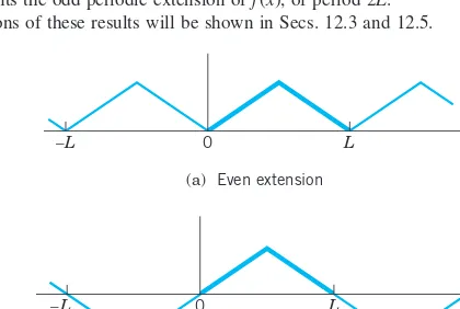
The section on Fourier series introduces the concept of representing periodic functions as infinite series of sine and cosine functions. This foundational idea is crucial for both engineers and applied mathematicians, as it allows for the simplification of complex periodic phenomena. The text begins by defining periodic functions, emphasizing the importance of the fundamental period, and illustrates how familiar functions like sine and cosine can be utilized in this context. The section also discusses the convergence of these series and the conditions under which they can be applied, making it clear that Fourier series can represent a broader class of functions compared to Taylor series, particularly those that are discontinuous. This is significant for educational objectives as it provides students with a tool for analyzing and approximating periodic functions in various applications.
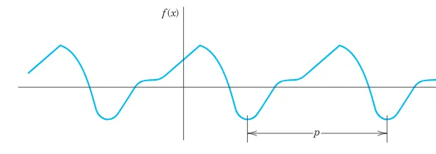
11.1.1 Definition of Periodic Functions
This subsection defines periodic functions and their fundamental period, establishing the groundwork for understanding Fourier series. It explains that a function is periodic if it can be repeated over intervals of a certain length, known as the period. The importance of this concept is highlighted through examples of common periodic functions like sine and cosine. Understanding periodicity is essential for students as it connects to real-world applications such as waveforms in engineering and physics.
11.1.2 Representation of Functions
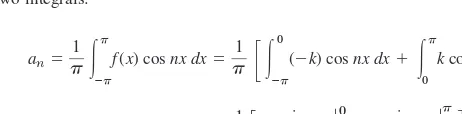
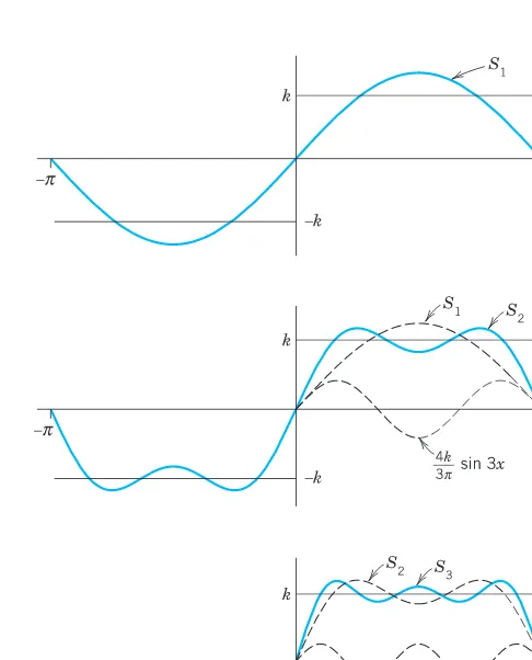
Here, the focus shifts to how periodic functions can be expressed as a sum of sine and cosine terms. The section presents the general form of a Fourier series and introduces Fourier coefficients, which are calculated using integrals. This mathematical formulation is crucial for students to grasp, as it bridges theoretical mathematics and practical application, allowing them to represent complex signals and systems in a manageable form.
11.1.3 Convergence of Fourier Series
This subsection addresses the convergence of Fourier series, detailing the conditions under which these series converge to the original function. It introduces the concept of piecewise continuity and discusses the implications of discontinuities on the convergence behavior of the series. This understanding is vital for students, as it informs them about the limitations and capabilities of Fourier series in practical scenarios, particularly in engineering applications.
11.1.4 Examples and Applications
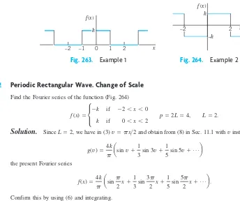
The section concludes with practical examples that demonstrate the application of Fourier series in solving real-world problems. It includes a detailed example of a periodic rectangular wave, showcasing how to derive Fourier coefficients and construct the corresponding Fourier series. This practical application reinforces the theoretical concepts and illustrates the utility of Fourier series in fields such as electrical engineering and signal processing, making the learning experience relevant and engaging.