SOLVING LINEAR GOAL PROGRAMMING
USING DUAL SIMPLEX METHOD
Elfira Safitri, Habibis Saleh and M. D. H. Gamal
Abstract. Linear goal programming is an extension of linear programming used
to solve a linear programming problem with more than one objective functions. In this article we study the dual simplex method to solve the goal programming. We slightly modify the step six of Schniederjans and Kwak [Journal of the Operational Research Society, 33(1982): 247-252] by performing Gauss-Jordan elimination to update a new table. The computational results for relatively small problems show that the dual method produces the same number of iterations as other methods.
1. INTRODUCTION
A simplex algorithm for solving linear programming problems was ini-tially developed by Dantzig [2] and later modified by Lee [5] for solving a linear goal programming. Lee [5] treats the full simplex tables, expanding the evaluation zjcj to a row for every preemptive priority. The selection
rules for this algorithms follow conventional primal linear programming. In an effort to reduce the computational time to find the solution of linear programming problems, Schniederjans and Kwaks [8] developed an alterna-tive simplex method based on Boumols simplex method. This dual simplex method removes up to one half of the columns in the table simplex deviation. Olson [6] compares four methods of goal programming: Schniederjans and Kwaks [8], Lee [5], Arthur and Ravindran [1] and Olson [6]. Olson
Received 12-11-2014, Accepted 15-12-2014.
2010 Mathematics Subject Classification: 90C29
Key words and Phrases: Dual simplex method, Gauss-Jordan elimination, Goal programming.
[6] also presents the revised simplex method to solve the problem of goal programming utilizing Schniederjans and Kwaks dual simplex procedure to compute a new table element. Olsons results can be summarized that the dual simplex method is superior than the revised simplex method, the method presented by Lee [5] and Arthur and Ravindran [1].
Olson [6] also illustrates the major limitations in applying the method, i.e. the lack of the algorithm that is able to reach a solution in a reasonable computational time. The most commonly used solution methods of goal programming was introduced by Lee [5] and Ignizio [4] based on the simplex method of Dantzig [2]. Both methods require a column in the simplex table for positive and negative deviation variables. The most commonly methods used to accomplish goal programmings are the modified simplex method, the preemptive method, the non-preemptive method and the revised simplex method.
In this article the authors discuss the dual simplex method. The pur-pose of this article is to present an alternative simplex method to solve the goal programming problems. The dual simplex method is the basis of this alternative method with slight modifications in step six of Schniederjans and Kwak [8], namely the completion step. In the previous study Schniederjans and Kwak [8] update the new tables using multiplication formula of two corner elements, whereas the authors use the Gauss-Jordan elimination to update them. In particular, this paper presents the steps of the dual simplex method and illustrates the method with a numerical example.
2. SOLUTION PROCEDURE
where z is the sum of the deviations from all desired goals having m goal constraints and n decision variables xj and wi are non-negative constants
representing the relative weight to be assigned to the deviational variables
d−
i and d
+
i for each goal constraint. The Pi are the preemptive priorities
assigned to sets of goals that are grouped together in the problem formula-tion. The constants aij are the ones attached to each decision variable and
thebi are the right-hand-side values or goals of each constraint.
The way we set up the initial table for this goal programming problem is the same fashion as the ordinary linear programming problem table. The
d+i variables written as follows:
d+i =−bi+ n
X
j=1
aijxj+d−i ;i= 1,2, . . . , m,
are used as their initial basic variables. For the sake of the initial table for-mulation, a zero priority is artificially assigned in the absence of a variable
d+i in a goal constraint. Table 1 presents an initial table. The decision vari-ablesxj and negative deviational variablesd−i are labeled in Row 1. These
variables are non-basic variables whose values are zero. The coefficients of the decision variables, aij, are placed in column 3 and an identity
ma-trix is placed in column 4 representing the inclusion of negative deviational variables, and the right-hand-side (RHS) values, bi are placed in column 5.
The appropriate priority factors Pi and weights wi for each positive
deviational variable (i.e. basic variables) are listed in column 1 of Table 1, including artificial deviational variables as shown in column 2. Row 2, column 5 in the table contains a value called total absolute deviation. It represents the amount of total deviations from all goals for each table as the iterative process proceeds. Row 2, column 3 is simply a row vector of zero representing the inclusion of all decision variables in the computational process. The appropriate weights wi for each negative deviational variable
included in the objective function are listed in Row 2, column 4. The pro-cedure for generating the next table is based on the modified Gauss-Jordan method given as follows (Schniederjans and Kwaks [8]):
1. Determine the leaving variable. This is accomplished by selecting the variable with the highest-ranked priority (P0 > P1 > P2 > . . . > Pn). When two or more variables have the same priority ranking, the
Table 1: Initial table for the alternative model
2. Determine the entering variable. This is accomplished by selecting the column that has the largest coefficient in the pivot row. The corresponding column is called the pivot column. The element in the intersection of pivot row and pivot column is called a pivot element.
3. Exchanging the variables in the pivot row and pivot column.
4. In the new table, the new element that corresponds to the pivot ele-ment is found by taking the reciprocal of the pivot eleele-ment. All other elements in the row are found by dividing the pivot-row elements by the pivot element and changing the resulting sign.
5. Perform Gauss-Jordan elimination to update the new table.
New row = old row (pivot column coefficient ×the new row of pivot-table)
6. Determine the new total absolute deviation by the following formula:
z=X|wibi|
7. Check to see if the solution is optimal.
The solution is optimal if the basic variables are all positive and the preemptive priority rule is satisfied. If one or more of the basic vari-ables are negative, repeat steps 1 to 8. If all the basic varivari-ables are positive but the preemptive priority rule is not satisfied, the solution is not optimal. Continue to step 9.
8. Determine which variable is to exit the solution basis.
9. Determine which variable is to enter the solution basis.
This is accomplished by selecting the column that has smallest result-ing ratio when the negative coefficients in the pivot row are divided into their respective positive elements in row 2 changing the resulting sign. This variable labels the pivot column. Repeat steps 3 to 8.
10. The solution is optimal if the basic variables are all positive and one or more of the objective function rows (i.e. row 2) have a negative sign.
3. AN ILUSTRATIVE EXAMPLE
To illustrate the proposed goal programming method, the following problem is considered (Hillier-Lieberman [3]):
The first step that must be done is to change it into a standard form. The following is a dual form of goal programming:
minz= 5P1d−1 + 2P2d2++ 4P2d−2 + 3P3d+3 (1)
After converting into a dual form, we determine basic and non-basic vari-ables. For the dual simplex method, the basic variables are d+1, d+2 and d+3, whereas non-basic variables are x1, x2, x3, d1−, d−2 and d−3. After basic
Table 2: Initial table of dual simplex method
In Table 2, element 0 in the z row, corresponding to columns x1, x2
and x3, select the largest coefficient in the pivot row for a pivot column selection. Using this criterion we choose columns x3. Then, the first and
the second iteration are shown in Table 3 and Table 4 respectively.
Table 3: The first iteration table of dal simplex method
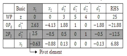
In Table 5, the basic variables are all positive but the preemptive priority is not satisfied yet, so repeat step 9. Determine which variable is to exit the solution basis. Determine which variable is to exit the solution basis by selecting the largest positive element in column 9 with the highest priority level. Because the highest priority only at d+3 sod+3 variable is to exit the solution basis.
Since all variables are positive and bases for all preemptive priority are satisfied, then the solution is optimal. Thus the optimal solution obtained is x1 = 8.33, x2 = 0, x3 = 1.67, d−
Table 4: The second iteration table of dual simplex method
Table 5: The third iteration table of dual simplex method
4. CONCLUSION
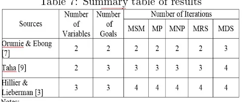
In this paper, to solve the dual form of the preemptive weighted prior-ity goal programming problem, the authors slightly modify the step six of Schniederjans and Kwak [8] by performing Gauss-Jordan elimination to up-date a new table. Particularly in the example of Hillier-Lieberman [3], the dual simplex method produces the same number of iterations as other four methods: modified simplex method, preemptive method, non-preemptive method and revised simplex method
Generally, the dual simplex method produces the same number of it-erations as other methods. However, Table 7 shows that the dual simplex method yield more iterations when compared to four other methods. A summary of the results of three examples is presented in Table 7.
Table 7: Summary table of results
REFERENCES
1. Arthur, J. L. and A. Ravindran. An efficient goal programming algorithm using constraint partitioning and variable elimination. Management Sci-ence,24(1978): 867-86.
2. Dantzig, G. B.Programming a Linear Structure. Comptroller, United Air Force, Washington, D. C.,1948.
3. Hiller, F. S dan Lieberman, G. J. Introduction Operation Research, Five Ed. , McGraw-Hill, New York, 1990.
4. Ignizio, J. P.Introduction to Linear Goal Programming, Sage Publication, California, 1986.
5. Lee, S. M.Goal Programming for Decision Analysis. Auerbach, Philadel-phia, 1972.
6. Olson, D. L. Comparison of Four Goal Programming Algorithm. Journal of the Operational Research Society, 35 (1984): 347-354.
7. Orumie, U. C and D. W. U. Ebong. Another Efficient Method of Solving Weighted Goal Programming. Asian Journal of Mathematics and Appli-cations,2013(2010):1-11.
8. Schniederjans, M. J dan N. K. Kwak. 1982. An Alternative Solution Method for Goal Programming Problems : A Tutorial. Jurnal of Opera-tion Research Society, 33 (1982): 247-252.
9. Taha, H.A. Operations Research: An Introduction, Seven Ed., Prentice-Hall, New Jersey, 2003.
Elfira Safitri: Islamic State University of Sultan Syarif Kasim, Indonesia.
E-mail: elfirasafitri [email protected]
Habibis Saleh: University of Riau, Indonesia.