Relevancy of Harrod Domar Model in Nepal

Relevancy of Harrod-Domar Model in Nepalese Economy Rajendra Adhikari, Ph.D.

Lecturer, Department of Economics Mechi Multiple Campus, Bhadrapur

Tribhuvan University, Nepal Abstract

Present paper aims at examining the relevance of Harrod-Domar model in Nepal through econometric techniques by using the data sets of saving, capital formation/capital output ratio and economic growth over the period 1974/75-2016/17. The variables, under study are found to be cointegrated, and there appears uni-directional causality running from saving to economic growth; and economic growth is found to be caused also by incremental capital output ratio as indicated by Granger causality test. The auto regressive distributed lag models report that economic growth of Nepal during the study period is affected positively by growth rate of saving; and incremental capital output ratio has the negative effect on economic growth, signifying the relevance of Harrod-Domar model in the economy of Nepal. This study plays crucial role in policy perspective that Government of Nepal should create the environment as to lead saving to increase, and saving should be converted into the capital formation through the development of capital market. Additionally, the capital substitution policy is indispensable to formulate through development of skilled labor force.

Introduction

A number of growth theories are available in macroeconomic literature to analyze the determinants of economic growth. According to classical economist Ricardo, labor is the only factor to determine agricultural output, and hence output is taken as the function of labor force, that is: Y=f(L) . On the other hand, Neo-Classical theory of Solow-Swan (1956) examined labor, capital and technology as the determinants of economic

growth, that is: Yt=Atf(Lt, Kt) . Keynes (1936) analyzed that level of employment and output are determined by aggregate effective demand and aggregate effective demand is, in turn determined by level of consumption demand and investment demand.

Investment is more powerful tool to determine income in the Keynesian economy.

Likewise, Samuelson (1948) and Hicks (1967) also emphasized on the role of investment to achieve high economic growth. However, Harrod (1939) and Domar (1946) declared that economic growth is determined by growth rate of saving and productivity of capital.

economic growth (Najarzadeh, Reed & Tasan ,2014). This view clearly implies that saving

plays influential role for capital formation to achieve steady-state growth in the economy. Harrod (1960, 1963a) revealed that the natural growth rate is exogenous in respect with the rate of saving. According to him, the optimum saving which is essential for implementing natural growth rate is an instrument to formulate macroeconomic growth policy in the context of the postwar welfare state. The Harrod-Domar growth Theory is the integration of Harrod (1939) and Domar (1946) growth models based on the

experience of capitalist economies. This theory examines the requirement of capital output ratio and growth rate of saving for the steady-state growth in the economy. This model laid its foundation to neo-Classical theory and utilized the Keynesian technique of multiplier assuming no excess capacity in the economy that planned saving equals planned investment (Grabowski & Shields, 2000). According to this model, there is direct link between economic growth and investment and saving is the main source for capital accumulation. Harrod-Domar model assumes that investment plays dual role: demand side role and supply side role. The Harrod-Domar model conspicuously emphasized the role of rate of saving and capital output ratio for enhancing economic growth.

Harrod-Domar model is one of the prominent models to analyze an economy’s growth rate as a function of growth rate of saving and productivity of capital. This model was independently developed by Harrod in1939 and Domar in 1946. Though Harrod and Domar developed their growth models independently similar conclusions were drawn that steady state growth could be attained at Razor’s Edge.

S=sY (1)

Where, s=¿ proportion of the income devoted for saving (0<s<1)

Capital Output Ratio (COR) is defined as the ratio capital stock to output/income, that is: K/Y=k (2)

⇒ ∆ K/∆Y=k

⇒k ∆Y=∆ K

⇒k ∆Y=I (3)

( ∴I=∆ K¿ The change in stock of capital is the investment I . There is no excess capacity in the economy, that is:

I=S (4)

⇒ k ∆ Y=sY

⇒ ∆ Y/Y=s/k (5)

Growth rate of output is determined jointly by COR and rate of growth of saving. Thus, it can be concluded that economic growth is the function of growth rate of saving and COR, that is:

G=f(s, k) (6)

Literature Review

A number of empirical studies are available in economic literature regarding the determinants of economic growth. Some studies found saving and investment/COR as important determinants of growth. Saving can be taken as one of the main sources of capital formation in the economy. As rate of capital formation increases, high economic growth can be attained in the economy. According to Abu (2010), increase in saving causes capital formation to increase and thereby high economic growth can be attained.

Jappelli and Pagano (1994), using Ordinary Least Square, found that higher growth rate of saving results higher economic growth. Mehanna (n.d.) attempted to explore the relationship between investment and economic growth in 80 developing countries for the period 1982-1997 and established a strong positive impact of investment on economic growth. In another study Moreira (2005) using Generalized Methods of Moments found economic growth is caused by saving. In the study of Dritsakis, Varelas, and Adamopoulos (2006) was observed the long run relationship among exports, gross capital formation, FDI and economic growth for Greece over the period 1960-2002. The authors employed multivariate vector autoregressive and found unidirectional causality running from gross fixed capital formation and economic growth.

economic growth in the economy of Bangladesh over the period 1986-2008 by employing cointegration test and Granger causality test. The test proved economic growth in Bangladesh was caused positively by capital formation and FDI.

Najarzadeh, Reed and Tasan (2014) by using the annual data over the period 1972-2010 and applying Autoregressive Distributed Lags (ARDL) and Error Correction Modeling (ECM), found a positive impact of saving on economic growth in the economy of Iran. Jagadeesh (2015) also examined the impact of saving on economic growth for Botswana applying ARDL Bound test for cointegration and found Harrod-Domar being applied. Conversely, Nwanne (2014) in his study for Nigeria found adverse effect of saving on economic growth as reported by cointegration test, VECM and Granger causality test, and hence inapplicability of Harrod-Domar model. However, economic growth was positively affected by capital formation in the study. Osundina and Osundina (2014) in their study observed the positive effect of saving and capital accumulation on economic growth in Nigeria, and hence the Harrod-Domar model was applicable in Nigerian economy.

Research Methodology

The present study seeks to analyze whether saving and investment/COR are the determinants of Nepalese economic growth through the econometric methodology. Augmented Dickey Fuller (ADF) unit root test, Johansen system of cointegration test, Granger causality test and auto regressive distributed lag (ARDL) models are the main econometric tools used in the present study. The ADF unit root test has been performed to identify the stationarity or non-stationarity of the variables and use the models

is applied to examine the long run relationship among the variables. Once the variables under study are cointegrated, Granger causality test has been used to observe the causal linkage between the variables. Finally, ARDL models are used to examine the impact of saving and COR on economic growth. .

ADF Unit Root Test

The estimable equation proposed for ADF unit root test is:

Δy_t=μ+γy_t−1+

∑

¿ j=1

p

α_jΔy_t−j+β_t+ε_t

¿ (7) Where, yt follows an AR (k) process. The constant term μ is said to be drift

term. In the equation (7), the notation t _{denotes the time trend, and} p _{is the lag}

length of the time series and ε_t is defined as white noise error term. The null

hypothesis for ADF unit root test is ‘The variable has a unit root’. Whether the variable has unit root or not can be confirmed with the help of t-statistic and corresponding probability value.

Johansen System of Cointegration Test

Johansen (1988) proposed a test for identifying the long run relationship between

and among the variables and number of cointegrating vector. For this, Let X_t be a

vector of N time series, each of which is I(1) variable, with a vector autoregressive (VAR) representation of order k ,

X

t

=

π

1

X

t−1

+

.. .. .

+

π

k

X

t−k

+

ε

t (8)

Where,

π

i _{are (N} ¿N _{) matrices of unknown constants and}

ε

t _{is an}

mean and variance matrix

∑

e _{i.e. N (0,}

∑

e _{). The estimable equation for the}

Two likelihood ratio tests have been proposed for the determination of the number of cointegrated vectors, which are: Maximum Eigen value test, and Trace statistic.

λmax=−Tln(1−λr+1) (10) Where,

λ

r+1

...

λ

n _{are the n-r smallest squared canonical correlations and T = the}

number of observations. The Maximum Eigen is given by,

λ

trace

=−

T

∑

ln

(

1

−

λ

_i

)

(11)

Granger Causality Test

Auto Regressive Distributed Lag (ARDL) Model

The ARDL model has been recommend in the spirit that variable y is affected by not only the value of x at the same time t but also by its lagged values plus

some disturbance term, x_t, x_t−1, xt−2….., xt−k, εt .this can be written in the functional form as:

x

y_t=f(¿¿t , xt−1, xt−2….., xt−k, εt) ¿

In linear form,

y_t=α+β₀x_t+β₁x_t−1+β₂x_t−2+…+β_jx_t−k+ε_t (14) The Ad Hoc approach popularized by Alt (1942) and Tinbergen (1949) has been used to identify the lags to be included in independent variable.

Data and Variables

Economic growth and saving. The GDP and gross domestic saving in real

terms and transformed into logarithmic form are represented by Y_t and S_t their

first differences by dYt and dSt respectively. The variables :dYt and

dS_t are taken as the proxy for economic growth and domestic saving of Nepalese

economy respectively.

Capital formation. Gross investment/ Gross Capital Formation in real terms

converted into logarithmic form is represented by I_t and its first difference by dI_t , which is taken as the proxy for capital formation of Nepalese economy.

Incremental capital output ratio. The productivity of Nepalese capital is

measured by incremental capital output ratio (ICOR). Fixed capital formation and GDP in real terms are used to calculate ICOR.

ICOR = (GFCt/GDPt)/(GDPt−GDPt−1/GDPt)

(15)

= GFC_t/GDP_t−GDP_t−1

where, GFC_t = Gross Fixed Capital in Real Terms at time ‘t’ GDP_t = Gross Domestic Product at time‘t’

GDP_t−1 = Gross Domestic Product at time preceding’

Data Analysis and Discussion of Results

ADF Unit Root Test

stationarity. Hence, the results from ADF unit root test have been presented through Table-1.

Table 1

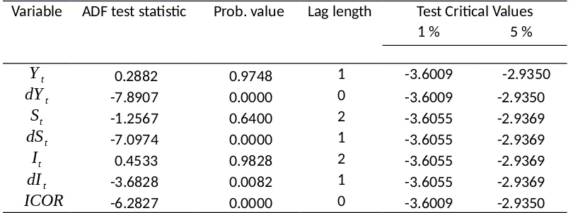
Augmented Dickey Fuller Unit Root Test on Variables

Variable ADF test statistic Prob. value Lag length Test Critical Values

1 % 5 %

Y_{t 0.2882 0.9748} 1 -3.6009 -2.9350

dY_{t -7.8907 0.0000} 0 _{-3.6009 -2.9350}

S_{t -1.2567 0.6400} 2 _{-3.6055 -2.9369}

dS_{t -7.0974 0.0000} 1 -3.6055 -2.9369

I_{t 0.4533 0.9828} 2 _{-3.6055 -2.9369}

dI_{t -3.6828 0.0082} 1 -3.6055 -2.9369

ICOR _{-6.2827 0.0000} 0 _{-3.6009 -2.9350}

From Table 1, it is observed that the null hypotheses ‘The variable has unit root’

are not rejected at level form for the variables: Y_t , S_t and I_t while considering

constant as exogenous as reported by the t-statistic at both 5 percent and 1 percent level of significance and corresponding probability values. On the other hand, there is no

reason to accept null hypotheses for all variables: dY_t , dS_t and dI_t in their first

differences including the variable ICOR . Thus, the variables except ICOR are non-stationary at level; whereas these variables including ICOR are stationary at their first differences.

Johansen’s Cointegration Test

and Trace statistic values. Table- 2 and Table-3 reveal the results from Johansen’s

cointegration test among the variables: Y_t , S_t and I_t .

Using first order VAR of the variables under investigation, the hypotheses of r=0 and r ≤1 are uniformly rejected in favor of the alternative hypothesis

r=1 and r=2 respectively employing the maximum Eigen-value test as reported by 4th _{column of Table-2, indicating two cointegrating vectors. Thus, on the basis of}

maximum Eigen-value test, the variables: Yt , St and It are found to be cointegrated. Table 2

Test Based on Maximum Eigen Value(

λ

max ₎

H₀ H_a λ_i λ_max 5% Critical

Value Probability

r=0 r=1 0.547664 56.75427 35.19275 0.0001

r ≤1 r=2 0.386529 24.22771 20.26184 0.0135

r ≤2 r=3 0.097239 4.194186 9.164546 0.3840

Table 3

Test Based on Maximum Eigen Value(

λ

max ₎

H₀ H_a λ_i λ_trace 5% Critical

Value Probability

r=0 r=1 0.547664 32.52656 22.29962 0.0013

r ≤1 r=2 0.386529 20.03352 15.89210 0.0105

r ≤2 r=3 0.097239 4.194186 9.164546 0.3840

Turning to the trace test as reported by Table-3, the null hypothesis r ¿ _{2 cannot}

Thus, both maximum Eigen value and Trace statistic specify that there appears cointegration among the variables under study.

Granger Causality Test

Since the variables: Y_t , S_t and I_t are found to be cointegrated as reported by Johansen’s cointegration test, the causal linkage between the variables are observed through Granger causality. Under Johansen’s cointegration test, the

non-stationary data sets of the variables: Y_t , S_t and I_t were used. However, under

Granger causality test the stationary variables dY_t , dS_t and ICOR are used. The

ICOR is used instead of I_t in Granger causality test in the spirit of Harrod-Domar model.

Table-4 portrays the results from Granger causality test. In which, the null

hypothesis ‘ ICOR does not Granger Cause dYt' at lag 1 and lag 3 is rejected at 10 percent and 5 percent level of significance respectively as reported by F-statistics and

corresponding probability values. Similarly, the null hypothesis ' dSt does not Granger Cause ICOR ' is also rejected. However, other null hypotheses are not rejected even at 10 percent level of significance. The results imply that there appears uni-directional Granger causality

running from ICOR to dYt . There is also a little economic significance between dSt

and ICOR for uni-directional Granger causality running from dSt to ICOR .

Table 4

Endogenous variables:

{

dYt,dSt∧ICOR

}

Null Hypothesis ( H0 : α=0 ) Lags F-statistic Probability ICOR does not Granger Cause

dY_t

dY_t does not Granger Cause

ICOR

dY_t does not Granger Cause

d S_t

dS_t does not Granger Cause

ICOR

dY_t does not Granger Cause

ICOR

dY_t does not Granger Cause

d S_t

dS_t does not Granger Cause

ICOR

The results from Granger causality could not testify in accordance with the spirit of Harrod-Domar model. It is because the saving could not Granger cause economic growth though capital output ratio could cause economic growth. Hence, the present study considers the raw data of GDP and saving in real terms and their first differences to apply granger causality. Real GDP and saving in their first differences are represented by

GDP_rt and S_rt respectively. However, incremental capital output ratio of fixed

capital ICOR is same as before.

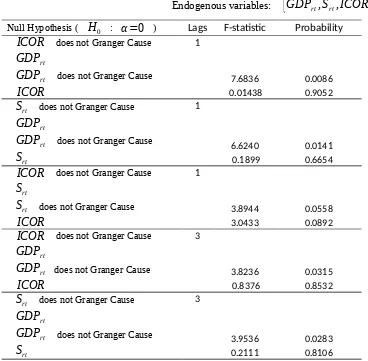
Table-5 depicts the results from Granger causality among the endogenous

' ICOR does not Granger Cause GDP_rt' at lag 1 and lag 3 is strongly rejected at 1

percent and 5 percent level of significance respectively. Whereas the null hypothesis ' GDP_rt does not Granger Cause ICOR ' is not rejected at both lag 1 and lag 3. This

implies uni-directional causality running from incremental capital output ratio to GDP. The saving is also found causing GDP at both lag 1 and lag 3 at 5 percent level of

significance. Whereas, GDP is not found causing saving at any lag. This also testifies uni-directional causality running from saving to GDP. Finally, ICOR is found saving causing at 10 percent level of significance at lag 1.

Table 5

Pair Wise Granger Causality Test

Endogenous variables:

{

GDP_rt, S_rt, ICOR

}

Null Hypothesis ( H0 : α=0 ) Lags F-statistic Probability ICOR does not Granger Cause

GDP_rt

GDP_rt does not Granger Cause

ICOR

S_rt does not Granger Cause

GDP_rt

GDP_rt does not Granger Cause

S_rt

S_rt does not Granger Cause

ICOR

S_rt does not Granger Cause

GDP_rt

GDP_rt does not Granger Cause

ICOR does not Granger Cause

S_rt

S_rt does not Granger Cause

ICOR

3

0.0658 1.7223

0.9364 0.1934

Autoregressive Distributed Lag Model

For ARDL model, the present study has used the variables dY_t, d S_t, and

ICOR in which dY_t is taken as dependent variable, and d S_t, ICOR independent

variable. First dY_t is regressed on d S_t applying Ad Hoc approach. The dependent

variable dYt is regressed on the independent variable d St at lag 0 and 1. The

coefficient of d S_t at lag 1 is not found statistically significant. Moreover, the

coefficient of d S_t is found negative, against the priory assumption. Hence, the

dependent variable is regressed on with independent variable d S_t dropping it at lag 1 with ARDL model as represented by equation (14).

dY_t=α+βd S_t (16)

After replacing the parameters α and β by their values, equation (16) is converted as:

dY_t=0.0426+0.036d S_t (17)

[11.8248] [2.8176]1

(0.0000) (0.0075)2

In equation (17), the coefficient of d S_t is positive and significant at 0.01 as reported by t-statistic and corresponding probability value implying 1 percent increase in growth of saving causes economic growth to increase by 0.036 %.

Next, when dY_t is regressed on ICOR at lag 0, the coefficient of ICOR is

negative and statistically significant. Similarly, dY_t is regressed on ICOR at lag 0 and lag 1. The coefficient of ICOR at lag 1 is statistically significant but algebraic sign changes from negative to positive. It is not supported by theory. The theory states that economic growth varies inversely with ICOR. Hence, in accordance with Ad Hoc

approach, dY_t should be regressed on ICOR at lag 0 as represented by equation (16).

dYt=γ + θ ICOR (18)

Substituting the values of the parameters, equation (18) can be expressed as:

dY_t=0.0515 -0.001 ICOR

(19)

[12.0076] [-2.9736] (0.0000) (0.0050)

In equation (19), the coefficient of ICOR is negative and significant at 0.1 level. This

implies that higher incremental capital output ratio is accompanied by lower economic growth.

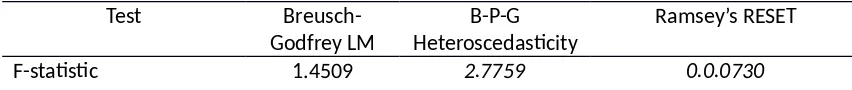
The robustness of the estimated OLS equations (17) and (19) under ARDL model has been testified through applying serial correlation test and heteroscedasticity test. Moreover, the stability of the estimated coefficients in the equations is testified by Ramsey’s RESET test. Breusch-Godfrey approach and Breusch-Pagan-Godfrey (B-P-G) approach are used to check the serial correlation and heteroscedasticity respectively in the residuals of the estimated OLS regression equations. Table-6 and Table-7 present the results from Breusch-Godfrey LM test, Breusch-Pagan-Godfrey heteroscedasticity test and Ramsey’s RESET test for equation (17) and (19) respectively.

From Table-6 it is observed that F-statistic, value of 3_{( T × R}2 _{) and probability}

value of χ2 (1) under Breusch-Godfrey Serial Correlation LM test imply that the null

hypothesis of no serial correlation is not rejected. Hence, the residuals of estimated equation (17) are not serially correlated. Likewise, the residuals are also free from

heteroscedasticity problem as accounted by F-statistic, value of (T × R2) and

corresponding probability value of χ2 _{(1) under B-P-G. Finally, as reported by}

t-statistic, F-statistic and Likelihood ratio of Ramsey’s RESET test, the estimated equation (17) is correctly specified bearing the property of linearity and hence it is stable equation. Table 6

Residuals Diagnostic and Stability Test of Estimated Equation of Equation (17)

Test Breusch-Godfrey

0.1176 0.9229 t-stat DF Probabilit y

0.3931 (39) 0.6963 Likelihood Ratio Stat. DF Probability 0.1661 (1)

As in Table-6, Table-7 also implies that the residuals of estimated equation (19) are not serially correlated and free from heteroscedasticity problem as specified Breusch-Godfrey serial correlation test and B-P-G heteroscedasticity test respectively. Finally, the estimated equation (19) is found to be correctly specified bearing the property of linearity and hence it is stable equation.

Table 7

Residuals Diagnostic and Stability Test of Estimated Equation of Equation (19)

Breusch-Degree of freedom (1,39) (1,40) (1,39)

Probability 0.2356 0.1035 0.7884

T × R2 1.5064 2.7255 t-Test

Probability χ2 _{(1) 0.2197 0.0988 t-stat DF Probabilit}

y 0.270

2 (39) 0.7884 Likelihood Ratio Stat. DF Probability

0.078

5 (1) 0.7793

Conclusions and Policy Implications

Present study confirms the long run relationship among the variables economic growth, saving and fixed capital formation, and there appears uni-directional Granger causality running from growth rate of saving to economic growth and incremental capital output ratio to economic growth in the economy of Nepal during the study period.

Growth rate of saving has positive impact on economic growth, which supports Harrod-Domar model and other subsequent researches. On the other hand, the

incremental capital output ratio has the negative impact on economic growth. This also supports Harrod-Domar model and other successive studies. Hence, Harrod-Domar model is found to be relevant in Nepalese economy.

Present study gives important feedback in policy perspective that economy should give focus on saving. However, saving alone cannot bring positive impact in the economy unless it is converted into the effective capital formation. For this, Government should give attention in the development of capital market. The incremental capital output ratio for the economy during the study period is found to be 6.94_{, which is very high as}

compared to World’s incremental capital output ratio around 3.0 for developed countries.

So, this high incremental capital output ratio of Nepalese economy is essential to reduce through substitution of capital by labor. However, Nepalese labor market lacks skilled labor dominated by unskilled and semi-skilled labor, not supportive to substitute capital and enhance high economic growth. That is why, Government of Nepal should give special attention in the development of skilled labor force in such a way as to substitute capital, and thereby reduce high incremental capital output ratio.

Reference

Abu, N. (2010).Savings and economic growth nexus in Nigeria: Granger causality and cointegration analysis. Review of Economic and Business Studies, 3(1), 93-104. Adhikary, B.K. (2011). FDI, trade openness, capital formation, and economic growth in

Bangladesh: a linkage analysis. International journal of Business Management, 6(1), 16-28.

Dickey, D. A., & Fuller, W. A. (1979). Distribution of estimates of autoregressive time series with unit root. Journal of the American Statistical Association, 427–431. Domar, E. (1946). Capital expansion, rate of growth and employment. Econometrica,

14, 13747.

Dritsakis, N., Varelas, E., & Adamopoulos, A. (2006). The Main Determinants of Economic Growth: An Empirical Investigation with Granger Causality Analysis for Greece. European Research Studies,9 (3-4), 47-58.

Grabowski, G., & Shields, M. (2000). A dynamic, Keynesian model of development. Journal of Economic Development, 25(1), 1-15.

Gujrati, D. N., Porter D.C., and Gunasekar, S. (2009). Basic econometrics. New Delhi, McGraw Hill Education Pvt. Ltd.

Harrod, R. F. (1960). Second essay in dynamic theory. Economic Journal, 70, 277-293. Harrod, R.F. (1963a). Themes in dynamic theory. Economic Journal, 73, 401-421. Harrod, R. F. (1939). An essay in dynamic theory. Economic Journal,49: 1433.

Hicks, J. R.(1967). Mr. Keynes and the Classics: A Suggested Interpretation. In: Readings in Macroeconomics. Edited Mueller, M. G., (ed), New York 1967.

Houthakker, H.S. (1965). On some determinants of saving in developed and

underdeveloped countries. In E. A. G. Robinson, (Ed.), Problems in economic development, (pp. 212-224). London, Macmillan.

Jagadeesh, D. (2015). The impact of savings in economic growth: an empirical study based on Botswana. International Journal of Research in Business Studies and Management, 2 (9),10-21.

Jappelli, T., & Pagano, M. (1994). Savings, growth and liquidity constraints. Quarterly Journal of Economics, 109, 83–109.

Johansen, S. (1988). Statistical analysis of cointegration vectors. Journal of Economic Dynamics and Control, 12, 231-254.

Keynes, J. M. (1936). The general theory of employment, interest and money. London, Macmillan, (Reprinted 2007).

Mehanna, R.A. (nd). The temporal causality between investment and growth in

Mehta, R.A. (2011). Short-run and long-run relationship between capital formation and economic growth in India. UMT, 19(2), 170-180.

(Ministry of Finance [ MOF], 2017). Economic survey (2016/17). Kathmandu.

Modigliani, Franco, (1970). The life-cycle hypothesis and inter-country differences in the saving ratio. In W. A. Eltis, M. FG. Scott, and J. N. Wolfe, (Eds.), Induction, growth, and trade: essays in honor of Sir Roy Harrod (pp. 197-225). Oxford, Oxford University Press.

Moreira, S. B. (2005). Evaluating the impact of foreign aid on economic growth: A cross-country study. Journal of Economic Development, 30(2), 25–48.

Najarzadeh, R., Reed, M., & Tasan, M. (2014). Relationship between saving and economic growth: the case for Iran. Journal of international Business and Economics. 2(4), 107-124.

Nwanne, T.F.I, (2014). Implication of saving and investment on economic growth in Nigeria. International Journal of Small Business and Entrepreneurship Research, 2 (4), 74-86.

Osundina, J.A., & Osundina, K.C. (2014). Capital Accumulation, Saving and Economic growth of a Nation- Evidence from Nigeria. Global Journal of Interdisciplinary Social Science, 3(3), 151-155.

Samuelson, P.A. (1948). Economics: an introductory analysis. New York: McGraw-Hill Book Company, Inc.

Sunny, I. O., & Osuagwn, N.C. (2016, April). Impact of capital formation on the economic development of Nigeria. Fifth International Conference on Global Business, Economics, Finance and Social Sciences. GB16 Chennai Conference, Chennai-India. Retrieved from

http://globalbizresearch.org/Chennai_Conference_2016_April/docs/conf %20paper/1.%20Global%20Business,%20Economics%20&

%20Sustainability/CF610.pdf

Swan, T. (1956). Economic Growth and Capital Accumulation. Economic Record. 32, 33461.