Validation of ANUGA hydraulic model using exact solutions to shallow water wave problems.

(1)

Validation of ANUGA hydraulic model using exact solutions to shallow water wave problems

This article has been downloaded from IOPscience. Please scroll down to see the full text article.

2013 J. Phys.: Conf. Ser. 423 012029

(http://iopscience.iop.org/1742-6596/423/1/012029)

Download details:

IP Address: 150.203.32.206

The article was downloaded on 15/04/2013 at 13:21

Please note that terms and conditions apply.

(2)

Validation of ANUGA hydraulic model using exact

solutions to shallow water wave problems

S Mungkasi1,2 _{and S G Roberts}1

1

Mathematical Sciences Institute, The Australian National University, Canberra, Australia

2

Department of Mathematics, Sanata Dharma University, Yogyakarta, Indonesia

E-mail: sudi.mungkasi@anu.edu.au, stephen.roberts@anu.edu.au

Abstract. ANUGA is an open source and free software developed by the Australian National University (ANU) and Geoscience Australia (GA). This software is a hydraulic numerical model used to solve the two-dimensional shallow water equations. The numerical method underlying it is a finite volume method. This paper presents some validation results of ANUGA with respect to exact solutions to shallow water flow problems. We identify the strengths of ANUGA and comment on future work that may be taken into account for ANUGA development.

1. Introduction

Shallow water flows have been studied mathematically since the ninteenth century. One available mathematical model is the shallow water equations derived by de Saint-Venant [5]. Based on the shallow water equations, a well-known solution to a dam break problem was derived by Ritter [16]. More comprehensive study of shallow water flows has been conducted by other authors, such as Stoker [19, 20].

Nowadays, the shallow water equations are widely applied to model river flows, tsunami inundations, and floods. However, the exact analytical solutions to the shallow water equations are available only for some specific cases. Numerical solutions are then desired as approximations of the exact solutions. Due to the applications of the shallow water equations, numerical packages (softwares) to solve these equations have been made available. Some of the softwares are commercial and some are free. One available free software is ANUGA. ANUGA is an open source software developed by the Australian National University (ANU) and Geoscience Australia (GA).

This paper validates ANUGA with respect to some exact analytical solutions to the shallow water equations. We identify the strengths of ANUGA when used to simulate shallow water flow problems. Comments on ANUGA shall also be provided for consideration on ANUGA development.

This paper is organised as follows. We provide a brief review of ANUGA software in Section 2. Some exact analytical solutions to the shallow water equations are collected in Section 3. In Section 4, we present numerical results of ANUGA experiments in comparison to the exact analytical solutions. Section 5 concludes this paper with some remarks.

(3)

2. ANUGA software

ANUGA is written in Python programming language for the User Interface together with C programming language for the expensive computation parts. Python gives a flexible interface, while C leads to fast computations. The combination of these two languages make ANUGA a robust software. This shall be demonstrated in the numerical experiments we present in Section 4.

The mathematical background underlying ANUGA is a finite volume method used to solve the two-dimensional shallow water equations. A description of it can be found in some documents, such as the ANUGA User Manual [18] and our previous work [11].

ANUGA has advantages for simulation of shallow water flows or waves. First, it can be used to simulate tsunami, dam break, flood inundations and other types of shallow flows. Second, it can handle wetting and drying processes reasonably. Third, it is able to accurately resolve discontinuous water surface and velocity profiles, such as shock waves or hydraulic jumps. See previous publications [1, 3, 4, 6, 7, 8, 15, 17, 22, 23] about ANUGA for more detailed explanations on these advantages.

However, ANUGA has some limitations due to the implemented mathematical model [6]. First, it is not able to simulate turbulence and breaking waves. (To simulate turbulence and breaking waves, the Navier-Stokes equations or the three-dimensional shallow water equations should be used.) Second, ANUGA does not cover sedimentations, erosions and debris-type flows. Third, for simulating tsunamis, a sea floor displacement is not handled by ANUGA. (A tsunami generation should be taken into account for another model, such as Method of Splitting Tsunamis (MOST) and the URS Corporation’s Probabilistic Tsunami Hazard Analysis [15].)

3. Some exact analytical solutions to the shallow water equations

In this section, we collect four analytical solutions to shallow water flow (wave) problems. The first three are analytical solutions to problems in one dimension. The fourth is an analytical solution to a problem in two dimensions. All of the analytical solutions can be implemented to test the performance of numerical methods used to solve two-dimensional problems.

In this paper,we use the following notations. For two-dimensional problems:

• x, y represent the two-dimensional spatial variables,

• trepresents the time variable,

• u=u(x, y, t) denotes the water velocity in thex-direction, that is, the x-velocity,

• v=v(x, y, t) denotes the water velocity in they-direction, that is, the y-velocity,

• h=h(x, y, t) denotes the water height (depth),

• z=z(x, y) denotes the topography elevation (bed),

• w=h+z is called the stage, and

• g is the acceleration due to gravity.

The momentum in thex-direction called thex-momentum is given byuh, and the momentum in the y-direction called the y-momentum is given by vh. The notations for one-dimensional problems are similar to those for two-dimensional problems, but note that variables y andv do not arise in one-dimensional problems.

3.1. Dam break involving a dry area in one dimension

In this subsection, we recall the analytical solution to a dam break problem in one dimension. The initial condition is described as follows. A dam wall is located at points x =x0. The

topography is horizontal. Water height on the left of the dam wall is h=h1, and on the right

(4)

For the case withx0 = 0 ,h1>0 , andh0 = 0 , the analytical solution to the dam break is as

follows. After the dam wall is removed (t >0) , the water height is

h(x, t) =

and the velocity is

u(x, t) =

The derivation of this analytical solution can be found in some references, such as Ritter [16], Stoker [19, 20], Mangeney, Heinrich, and Roche [10], as well as Mungkasi and Roberts [12, 13].

3.2. Dam break involving a shock wave in one dimension

Recall the dam break problem stated in the previous subsection. A dam wall is located at points

x=x0. The topography is horizontal. Water height on the left of the dam wall ish=h1, and

The derivation of this analytical solution can be found in some references, for example, Stoker [19, 20] and Mungkasi and Roberts [13].

3.3. Periodic wave on a sloping beach in one dimension

Consider a sloping beach with a positive constant slope. When the water is unperturbed, we have the dimensional setting: (i). the origin of the spatial domain is on the water surface, (ii). the horizontal distance of the water surface between the origin and the shoreline is L, (iii). the vertical distance (water depth or height) between the origin and the topography is h0.

(5)

One available analytical solution is as follows. The stage is

and the velocity is

u=₋AJ1

Note that this analytical solution is dimensionless, where the original dimensional quantities have been scaled [2, 9, 14]. The scalings are as follow:

• horizontal distances are scaled byL,

• vertical distances byh0, • time byL/√gh0, and • velocity by√gh0.

3.4. Periodic wave on a paraboloid channel in two dimensions

Now we consider a two-dimensional domain. We define parameters D0 = 1000 , L = 2500 , R0= 2000 such that

are the amplitude of oscillation at the origin, the angular frequency, and the period of oscillation. Furthermore, the topography is given by

z(x, y) =₋D0 1−

One available analytical solution is as follows. The water height is

h(x, y) = D0

In polar coordinates (r, θ) , the velocity ur in r-direction and the velocity uθ inθ-direction are

given by

ur= ωrAsin (ωθ)

2 [1₋Acos (ωθ)], (14)

uθ = 0. (15)

(6)

4. Computational experiments on problems in two-dimensional settings

In this section, we present our computational results. The results regard validations of ANUGA using exact solutions to shallow water flow (wave) problems. Note that we use the four analytical solutions presented in the previous section as the benchmarks. Some of those analytical solutions are for one-dimensional problems originally, but they can also be used to test two-dimensional numerical methods.

The numerical setting is as follows. The second order method is used. The spatial domain is discretised using the rectangular_cross function available in ANUGA. Quantities are measured in SI units. The acceleration due to the gravity is taken as g = 9.81 . The friction term is set to be zero.

Four computational experiments are performed. Results for a planar dam break involving a dry area are presented in Subsection 4.1. In Subsection 4.2, results for a planar dam break involving a shock wave are provided. Subsection 4.3 presents results for a periodic wave on a sloping beach. Finally, results for a periodic wave on a paraboloid channel are summarised in Subsection 4.4.

4.1. Planar dam break involving a dry area

We consider the spatial domain _{(x, y)_|x_∈ [₋60,60], y _∈ [₋10,10]_}. It is descretised into 100 by 20 rectangular-crosses, in which each rectangular cross has four uniform triangles. Therefore, we have 8000 triangles as the discretisation of the spatial domain. The dam wall is at x = 0 . Still water of height 10 is on the left of the dam wall and dry area is on the right of the dam wall.

The numerical solutions of the stage are shown in Figures 1, 3, and 5 for time t = 0,1,2 respectively. The corresponding x-momenta are depicted in Figures 2, 4, and 6 respectively. From these figures, we see that the numerical solutions match well with the analytical solution. However, a small inaccuracy around wet/dry interface occurs.

4.2. Planar dam break involving a shock wave

Recall the spatial domain and its discretisation used in the previous subsection, but now with a different initial condition. Taking the initial condition as still water of height 10 on the left of the dam wall and of height 1 on the right of the dam wall, we have a shock wave which involves in the solution after dam wall is removed.

The numerical solutions of the stage are shown in Figures 7, 9, and 11 for time t = 0,1,2 respectively. The corresponding x-velocities are depicted in Figures 8, 10, and 12 respectively. From these figures, the numerical solutions match well with the analytical solution. In addition, the shock wave is resolved accurately. It is interesting to see that diffusion is more visible around the rarefaction than around the shock. It suggests that the limiter implemented in ANUGA works very well for the second order method that we test in resolving the shock.

4.3. Periodic wave on a sloping beach

We consider the spatial domain_{(x, y)_|x_∈[0,55000], y_∈[0,500]_}. It is descretised into 550 by 5 rectangular-crosses, in which each rectangular cross has four uniform triangles. Therefore, we have 11000 triangles as the discretisation of the spatial domain.

We set some required parameters. The dimensional parameters are as follows:

• the reference length isL= 5_·104

,

• the reference depth is h0 = 5·102, • the period of oscillation is Tp = 9_·102

, and

• the amplitude at origin isa= 1.0 .

(7)

−60 −40 −20 _Position0 20 40 60

Figure 1. Stage of a cross section of the

planar dam break involving a dry area at

t= 0 .

Figure 2. x-momentum of a cross section

of the planar dam break involving a dry area at t= 0 .

t= 1 .

of the planar dam break involving a dry area at t= 1 .

t= 2 .

(8)

−601 −40 −20 _Position0 20 40 60

planar dam break involving a shock wave att= 0 .

Figure 8. x-velocity of a cross section

of the planar dam break involving a shock wave att= 0 .

(9)

0 10000 20000 30000 40000 50000 60000 −4

−2 0 2 4

Stage at several instants in time numerical

analytical

Carrier-Greenspan periodic wave at several instants in time (t = kTp/6 where k = 55, ...,60).

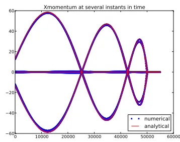
0 10000 20000 30000 40000 50000 60000 −60

−40 −20 0 20 40

60 Xmomentum at several instants in time

numerical analytical

of the Carrier-Greenspan periodic wave at several instants in time (t = kTp/6 where

k= 55, ...,60).

For the periodic wave on a sloping beach, we use the notation Tp for the dimensional period of

oscillation and the notationTfor the dimensionless one. The dimensionless parameters are found by some scalings as described in Subsection 3.3. We set the following dimensionless parameters:

• perturbation at origin

ǫ= a

h0

, (16)

• period of oscillation

T = Tp

√ gh0

L , (17)

• amplitude at shoreline

A= ǫ

J0(4π/T)

, (18)

whereJ0 is the Bessel function of the first kind of order 0 . See our previous work [14] for more

detailed dimensional and dimensionless settings.

The numerical solutions for the stage and x-momentum are shown in Figures 13 and 14 respectively at time t = kTp/6 where k = 55, ...,60 . These numerical solutions are found by considering the initial condition given by the analytical solution set up at timet= 0 . Based on these results, ANUGA can handle long waves accurately. The errors for the stage and momentum are indeed seen to be negligible.

4.4. Periodic wave on a paraboloid channel

Now we consider the spatial domain _{(x, y)_|x _∈ [₋4000,4000], y _∈ [₋4000,4000]_}. It is descretised into 100 by 100 rectangular-crosses, in which each rectangular cross has four uniform triangles. Therefore, we have 4_·105

(10)

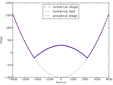
−4000 −3000 −2000 −1000 0 1000 2000 3000 4000 Position

−1000 −500 0 500 1000 1500 2000

Stage

numerical stage numerical bed analytical stage

water oscillation on a paraboloid channel at timet= 3.75T.

0 50 100 _Time150 200 250 300 −600

−400 −200 0 200 400 600 800

Stage

numerical analytical

Figure 16. Stage corresponding to the

origin of the spatial domain for time t = 0, ...,5T.

the physical energy of this smooth flow decreases over time. One way to reduce the damping or the loss of the physical energy is by running the code with a large number of rectangular crosses (hence a large number of triangles for the spatial domain discretisation), but this leads to an expensive computation.

5. Conclusions

ANUGA has been found to be a stable and robust software to simulate shallow water flows or waves. It can handle wetting and drying process and solve problems with shock waves accurately. For a very long running time, however, it seems that there exists a loss of physical energy, even when the flow is smooth and frictionless. A possible future development of ANUGA is to minimise this loss of physical energy of a smooth and frictionless flow with a reasonably cheap computation.

Acknowledgments

This work was financially supported by The Australian National University (ANU). The authors thank Mathew Langford at the ANU for proofreading the earlier version of this paper.

References

[1] Baldock T E, Barnes M P, Guard P A, Hie T, Hanslow D, Ranasinghe R, Gray D, and Nielsen O 2007 Modelling tsunami inundation on coastlines with characteristic formProc. 16th Australasian Fluid Mechanics Conf. (AFMC)939–942 AFMS.

[2] Carrier G F and Greenspan HP 1958 Water waves of finite amplitude on a sloping beachJournal of Fluid Mechanics4_97–109.

[3] Cousins W J, Power W L, Destegul U Z, King A B, Trevethick R, Blong R, Weir B, and Miliauskas B 2009 Earthquake and tsunami losses from major earthquakes affecting the Wellington regionProc. 2009 New Zealand Society for Earthquake Engineering Conf.paper number 24 NZSEE.

[4] Davies G 2011 A well-balanced discretization for a shallow water inundation model Proc. MODSIM 2011 Int. Congress on Modelling and Simulation2824–2830 MSSANZ.

[5] de Saint-Venant A J C B 1871 Theorie du mouvement non-permanent des eaux, avec application aux crues des rivieres et a l’introduction des marees dans leur litsComptes Rendus de l’Academie des Sciences, Paris

73147–154, 237–240.

[6] Floth U, Vott A, May S M, Bruckner H, and Brockmuller S 2009 Geo-scientific evidence versus computer models of tsunami landfall in the Lefkada coastal zone (NW Greece)Marburger Geographische Schriften

145_{140-156 (Marburg: Selbstverlag).}

(11)

[7] Jakeman J D, Bartzis N, Nielsen O, and Roberts S 2007 Inundation modelling of the December 2004 Indian Ocean tsunamiProc. MODSIM 2007 Int. Congress on Modelling and Simulation1667–1673 MSSANZ. [8] Jakeman J D, Nielsen O M, Putten K V, Mleczko R, Burbidge D, and Horspool N 2010 Towards spatially

distributed quantitative assessment of tsunami inundation modelsOcean Dynamics601115–1138. [9] Johns B 1982 Numerical integration of the shallow water equations over a sloping shelfInternational Journal

for Numerical Methods in Fluids2253–261.

[10] Mangeney A, Heinrich P, and Roche R 2000 Analytical solution for testing debris avalanche numerical models

Pure and Applied Geophysics1571081–1096.

[11] Mungkasi S and Roberts S G 2011 A finite volume method for shallow water flows on triangular computational gridsProc. 2011 Int. Conf. Advanced Computer Science and Information System (ICACSIS)79–84 IEEE. [12] Mungkasi S and Roberts S G 2011 A new analytical solution for testing debris avalanche numerical models

ANZIAM Journal52_C349–C363.

[13] Mungkasi S and Roberts S G 2012 Analytical solutions involving shock waves for testing debris avalanche numerical modelsPure and Applied Geophysics169_1847–1858.

[14] Mungkasi S and Roberts S G 2012 Approximations of the Carrier-Greenspan periodic solution to the shallow water wave equations for flows on a sloping beachInternational Journal for Numerical Methods in Fluids

69763–780.

[15] Nielsen O, Sexton J, Gray D, and Bartzis N 2006 Modelling answers tsunami questionsAusGeo News831–5 Geoscience Australia.

[16] Ritter A 1892 Die fortpflanzung der wasserwellenZeitschrift des Vereines Deutscher Ingenieure36947-954. [17] Roberts S G, Nielsen O M, and Jakeman J 2008 Simulation of tsunami and flash floodsIn Bock H G et al

(Eds) Modeling, Simulation and Optimization of Complex Processes489–498 (Berlin: Springer-Verlag). [18] Roberts S, Nielsen O, Gray D, and Sexton J 2010 ANUGA User Manual Commonwealth of Australia

(Geoscience Australia) and the Australian National University.

[19] Stoker J J 1948 The formation of breakers and boresCommunications on Pure and Applied Mathematics1 1-87.

[20] Stoker J J 1957 Water Waves: The Mathematical Theory with Application (New York: Interscience Publishers).

[21] Thacker W C 1981 Some exact solutions to the nonlinear shallow water equationsJournal of Fluid Mechanics

107_499–508.

[22] Van Drie R, Milevski P, and Simon M 2011 Validation of a 2-D Hydraulic Model-ANUGA, to undertake hydrologic analysisProc. 34th Int. Association for Hydro-Environment Engineering and Research Congress 2011450–457 IAHR.

[23] Van Drie R, Simon M, and Schymitzek I 2008 2D Hydraulic modelling over a wide range of applications with ANUGAProc. 9th National Conf. on Hydraulics in Water Engineering23–26 Engineers Australia. [24] Yoon S B and Cho J H 2001 Numerical simulation of coastal inundation over discontinuous topography