UNIfication of accounts and marginal costs for Transport Efficiency
UNITE
Towards an evidence-based charging policy for transport infrastructure
17 – 18 September 2001
Venue: Ecole nationale des ponts et chaussées
Estimating Environmental Costs using the Impact Pathway Approach
Peter Bickel, Rainer Friedrich
Institut für Energiewirtschaft und Rationelle Energieanwendung
Universität Stuttgart, Germany
1
Introduction
Environmental costs of transport cover a wide range of different impacts, including the various impacts of emissions of a large number of pollutants and noise on human health, materials, ecosystems, flora and fauna. Marginal cost pricing of infrastructure use, which is a stated objective of the European Commission (see European Commission 1998) requires an approach that is capable of quantifying marginal costs. On the other hand, for purposes of accounting total costs have to be estimated as well. In the following, the Impact Pathway Approach is presented, which allows quantification of environmental costs for both purposes in a consistent way.
2
The Impact Pathway Approach
The Principle
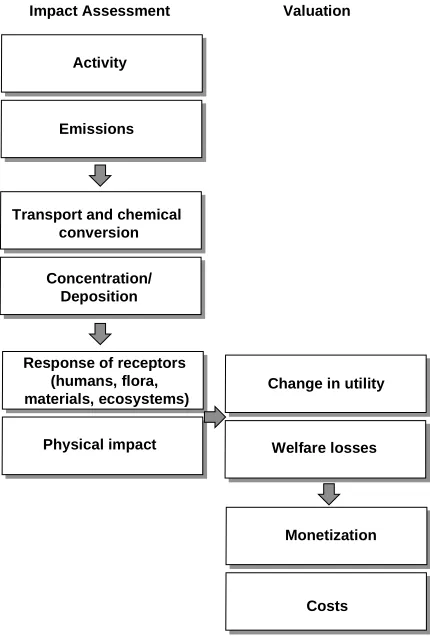
The Impact Pathway Approach (IPA) developed in the EC funded ExternE Project series (see Friedrich and Bickel 2001, European Commission 1999) meets these requirements. Figure 1 illustrates the procedure for quantifying impacts due to airborne pollutants: the chain of causal relationships starts from the pollutant emission through transport and chemical conversion in the atmosphere to the impacts on various receptors, such as human beings, crops, building materials or ecosystems. Welfare losses resulting from these impacts are transferred into monetary values. Based on the concepts of welfare economics, monetary valuation follows the approach of ‘willingness-to-pay’ for improved environmental quality. It is obvious, that not all impacts can be modelled for all pollutants in detail. For this reason the most important pollutants and damage categories (“priority impact pathways”) are selected for detailed analysis.
Activity
Emissions
Transport and chemical conversion
Concentration/ Deposition
Response of receptors (humans, flora, materials, ecosystems)
Physical impact
Change in utility
Welfare losses
Monetization
Costs Impact Assessment Valuation
Figure 1 The Impact Pathway Approach for the quantification of marginal external
costs caused by air pollution
It is important to note, that, although marginal costs are estimated, the emissions from all other sources and the background concentration influence the marginal change in concentration and deposition of the primary and secondary pollutants caused by the additional emissions; so all emissions and the resulting concentrations have to be accounted for in the framework. If emissions of pollutants and noise that occur in the future (or the past) have to be assessed, scenarios of the emissions and concentrations of pollutants at that time have to be used.
areas, the Impact Pathway Approach is widely recognised now as the most reliable tool for environmental impact assessment that - in contrast to other methodologies - allows the estimation of site specific marginal external costs, which is required to implement efficient pricing instruments. Appropriate models are available that support the standardised implementation of the complex impact pathway methodology with a reasonable effort.
Step 1: Emission modelling
The first step in the assessment procedure is the calculation of the emissions resulting from a transport activity. Based on parameters such as average speed, traffic situation, route gradient, load etc. emissions are calculated based on emission factors. Such emission factors have been compiled for road vehicles, diesel trains, ships and aircrafts within the MEET (Methodologies for estimating air pollutant emissions from transport) project.
For comparisons between modes, the system boundaries considered are very important. For instance, when comparing externalities of electric trains and passenger cars, the complete chain of fuel provision has to be considered for both modes. Obviously, it makes no sense to treat electric trains as having no airborne emissions from operation. Instead, the complete chain from coal, crude oil, etc. extraction up to the fuel or electricity consumption has to be taken into account.
Step 2: Dispersion modelling
Emissions of air pollutants are often transported over hundreds of kilometres, before they finally cause damage to human health or the environment. Although the marginal change in concentration decreases rapidly with increasing distance from the source, a substantial share of total damage occurs far away from the source, as the number of impaired persons, materials or plants increases at the same time.
To obtain marginal external costs, the changes in the concentration and deposition of primary and secondary pollutants due to the additional emissions caused by an additional vehicle trip have to be calculated. The relation between concentration and emission of pollutants is highly non-linear. So, air quality models that simulate as well the transport as the chemical transformation of pollutants in the atmosphere have to be used for the impact pathway approach. Of course, the results of air quality models, i.e. the concentration fields, depend on the weather situation. Also, deposition mechanisms may be affected by weather conditions. However, as long as it is not planned to implement weather-dependent prices, it is sufficient to calculate average concentration changes regarding the frequency of the different weather conditions. Depending on the range and type of pollutants considered different models are in use:
b) The Wind rose Trajectory Model (WTM) (Trukenmüller and Friedrich, 1995) is used to estimate the concentration and deposition of acid species on a European scale. WTM is a user-configurable Lagrangian trajectory model based upon a climatological approach that was first used by Derwent and Nodop (1986). The model differentiates between 24 sectors of the wind rose, such that from each sector a straight-line trajectory arrives at the receptor point. Concentrations at the receptor point are obtained by averaging over the results from these trajectories, suitably weighted by the winds in each 15° sector.
c) The Source-Receptor Ozone Model (SROM) which is based on source-receptor (S-R) relationships from the EMEP MSC-W oxidant model for five years of meteorology (Simpson et al., 1997) is used to estimate ozone concentrations on a European scale. Input to SROM are national annual NOxand anthropogenic NMVOC emissions data from 37 European countries, while output is calculated for individual EMEP 150x150 km2 grid squares by employing country-to-grid square matrices. To account for the non-linear nature of ozone creation, SROM utilises an interpolation procedure allowing S-R relationships to vary depending upon the emission level of the country concerned (Simpson and Eliassen, 1997, Appendix B).
The ECOSENSE model, an integrated impact assessment model developed within ExternE, integrates a)-c) of the above models together with databases covering receptor data (like population, land use etc.), meteorological data and emission data for the whole of Europe. Together with dose-response functions and monetary values stored in EcoSense, physical impacts and resulting (marginal) damage costs can be calculated within a consistent modelling framework, taking into account the information on receptor distribution. Impacts due to a point (e.g. a power plant) or line emission source are taken into account on a European scale, i.e. the dispersion of pollutants and related impacts are followed up throughout Europe.
A model for calculating noise dispersion, based on the German noise protection manuals for road (“RLS90”) and rail (“Schall 03”) completes the range of required models.
Step 3: Quantification of physical impacts
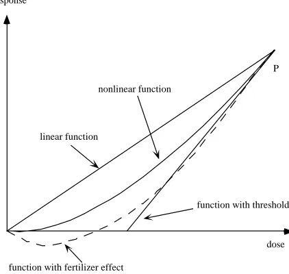
dose response
linear function
function with threshold nonlinear function
function with fertilizer effect
P
Possible behavior of dose-r esponse functions at low doses
Figure 2 A variety of possible forms for dose-response functions
E-R functions come in a variety of functional forms as illustrated in Figure 2. They may be linear or non-linear and contain thresholds (e.g. critical loads) or not. Those describing effects of various air pollutants on agriculture have proved to be particularly complex, incorporating both positive and negative effects, because of the potential for certain pollutants, e. g. those containing sulphur and nitrogen, to act as fertilisers.
Ideally, these functions and other models are derived from studies that are epidemiological - assessing the effects of pollutants on real populations of people, crops, etc. This type of work has the advantage of studying response under realistic conditions. However, results are much more difficult to interpret than when working under laboratory conditions, where the environment can be closely controlled. Although laboratory studies provide invaluable data on response mechanisms, they often suffer from the need to expose study populations to extremely high levels of pollutants, often significantly greater than they would be exposed to in the field. Extrapolation to lower, more realistic levels may introduce significant uncertainties, particularly in cases where there is reason to suspect that a threshold may exist.
Applicable exposure-response functions describing the impacts on human health, building materials, and crops are available for a range of pollutants, such as primary and secondary (i.e. nitrates, sulphates) particles, ozone, CO, SO2, NO2, benzene, etc. (see Friedrich and Bickel 2001). For more detailed background information on response functions see European Commission (1999). Only recently a set of exposure-response functions linking noise levels to health impacts became available.
Step 4: Monetary valuation
degradation). For health impacts such market prices do not exist. Therefore, monetary values for avoiding or reducing the risk of mortality and morbidity are derived from individual preferences revealed by market behaviour or by contingent valuation surveys. The “value of statistical life” (VSL) – or (to avoid misinterpretation) “value of a prevented fatality” (VPF) – is used in economic studies as a measure for welfare losses caused by risks to life. Mathematically, average willingness-to-pay (WTP) for a reduced mortality risk is divided by the risk reduction being valued (and, if this WTP refers to a risk for a group of more than one single person, also by the number of persons). E.g. if the average WTP for a risk reduction of 1 in 10,000 is 300€, the resulting VSL is 300€
divided by 1/10,000, that is 3 million€.
Though the valuation of mortality is often criticised from an ethical standpoint for putting monetary values on human lives (it is e.g. stated that people would value a certain human life infinitely high), reality shows that both public decision-makers and people themselves weigh the costs and benefits of investments in e.g. safety devices. And this very economic behaviour of people is the object of research in studies valuing risks to life and health. Values of mortality and morbidity risks are derived from individual preferences.
It is important here to emphasise that this value of statistical life represents an ex-ante perspective (that is, it refers to the statistical risks before the damage takes place), and not an ex-post perspective, i.e. it is not a measure for the life of a known individual or a certain death.
However, it has been questioned, whether it is appropriate to value all mortality risks with a uniform VSL, disregarding the loss of lifetime related to the risk. For example, it appears not justifiable to value the risk of premature death due to an increased PM10 concentration with the same value as the risk of dying in a traffic accident. While in the first case the average loss of life time is 9 months (i.e. mostly old persons with impaired health are affected), the age of an average traffic casualty victim is about 40 years, implying a loss of about 30 years of life time. Furthermore, additional increases in concentrations of pollutants might not only lead to impacts on additional persons not impaired before but also to a further reduction in lifetime by persons with already reduced life expectancy. In the latter case the use of the VSL approach will lead to inconsistencies.
Monetary values for risks of morbidity impacts can be estimated in analogy to mortality risks. But whereas for mortality risks the WTP component is dominating, in the case of morbidity risks the cost components “medical treatment” and “lost productivity” are more important. Costs of medical treatment and lost productivity – often called “costs of illness” (COI) – are easier to estimate, based on existing economic measures. However, as these figures do not reflect the full WTP of a person to avoid morbidity they should be used in addition to estimates of pain and suffering as far as available.
Quantification of Total Costs
Based on spatially disaggregated data on the emissions from a whole infrastructure network, total costs can be estimated with the impact pathway approach. Due to the sensitivity of the costs to the number of receptors near the emission source, spatial information is required for estimating the exposure of receptors resulting from the emissions. In the ideal case emissions are quantified based on infrastructure network maps together with the relevant transport activity data, such as the number and type of vehicles, the average speed and the relevant emission factors. From this data, emissions can be calculated with information on the location where the pollutants are emitted as required by the cost calculation procedure.
The calculation of the damages can be split into a local scale part and a regional scale part. As costs on the local scale are highly correlated with the number of receptors close to the emission source, a high level of resolution is required for the analysis. Based on a large number of case studies an equation for estimating local exposure can be derived by regression analysis. This allows to analyse a whole infrastructure network without carrying out detailed dispersion modelling which would be too expensive in terms of data collection and time. Instead, parameters characterising the population density in the vicinity of the route can be used to estimate exposure and costs. These parameters are calculated from the infrastructure network map and a corresponding population map. On the regional scale (which means here covering all of Europe) non-linearities due to air chemistry have to be considered. Furthermore, the geographical location, which determines the number of receptors affected, has important influence on the magnitude of costs. For instance pollutant emissions at the coast cause only little damage if pollutants are dispersed over the sea. To capture the non-linear effects of air chemistry costs have to be calculated with and without the total emissions of a transport mode or a vehicle category. The difference gives the costs caused by the respective mode or vehicle category.
3
Uncertainties and Gaps
The process of quantifying external costs involves considerable uncertainties, which arise from a number of sources, including:
• the variability inherent in any set of input data used for estimating external costs; • extrapolation of data from the laboratory to the field;
• assumptions regarding threshold conditions;
• lack of detailed information with respect to human behaviour and tastes; • assumptions like the selection of discount rate;
• the need to assume some scenario of the future for any long term impacts.
Generally speaking, the largest uncertainties are those associated with impact assessment and valuation, rather than quantification of emissions and other burdens. Furthermore, there are gaps, i.e. damage categories, where information e.g. on monetary valuation or exposure-response-relationships is lacking, so that no cost estimate can be provided. This means that the outcome of the use of the methods described here is not one specific value describing the external costs with certainty, but rather a range, within which the true value lies with a certain probability.
Despite these uncertainties, the use of the methods described here is seen to be useful, as - the knowledge of an order of magnitude of the environmental costs is obviously a
better aid for policy decisions than the alternative – having no quantitative information at all;
- the relative importance of different impact pathways is identified (e.g. has benzene in street canyons a higher impact on human health than fine particles?);
- the important parameters or key drivers, that cause high external costs, are identified; - the decision making process becomes more transparent and comprehensible; a
rational discussion of the underlying assumptions and political aims is facilitated; - areas for priority research are identified.
Furthermore, uncertainties in environmental cost estimates mostly reflect the uncertainties in our knowledge about e.g. impacts from air pollution and noise. This is correct and not a deficiency of the methodology – a scientific method cannot transfer uncertainty into certainty.
Clearly, the Impact-Pathway Approach is the appropriate method to quantify environmental costs. However, there are areas, where uncertainties are currently so high or where no quantitative information at all is available, so that even the order of magnitude of the damage cannot be estimated (e.g. global warming impacts). A possible method is the use of shadow prices. Shadow prices are inferred from reduction targets or constraints for emissions and estimate the opportunity costs of environmentally harmful activities assuming that a specified reduction target is socially desired. For global warming damages caused by the emission of CO2a shadow price for reaching the Kyoto reduction targets in the European Union is used, as long as reliable damage cost estimates are not available.
4
Summary
The impact pathway approach represents the state-of-the art methodology for estimating marginal and total (and thus average) environmental costs due to airborne pollutants and noise. Due to its bottom-up calculation principle site-specific impacts are taken into account. It can been used for quantifying environmental costs from all transport modes, from electricity production and other processes emitting airborne pollutants. The method has been used intensively to support decisions concerning a number of air quality directives of the European Commission (e.g. draft ozone directive, the national emissions ceiling directive, the draft directive for non-hazardous waste incineration, air quality guidelines on CO and benzene) and other international and national activities.
The user of the results has to be aware that uncertainties exist and certain assumptions have to be made. But this reflects uncertainties and gaps in our knowledge, and is not a deficiency of the methodology – a scientific method cannot transfer uncertainty into certainty.
5
References
Derwent, R.G. and K. Nodop 1986: Long-range transport and deposition of acidic nitrogen species in north-west Europe. Nature 324:356-358.
European Commission 1999: ExternE – Externalities of Energy, Vol.7: Methodology 1998 Update (EUR 19083). Luxembourg: Office for Official Publications of the European Communities.
European Commission 1998: Fair payment for Infrastructure Use: A phased approach to a common transport infrastructure framework in the EU. White paper. Brussels: European Commission
Friedrich, R. and P. Bickel (eds) 2001: Environmental external costs of transport. Berlin, Heidelberg, New York: Springer-Verlag
Simpson, D., K. Olendrzynski, A. Semb, E. Storen, S. Unger 1997: Photochemical oxidant modelling in Europe: multi-annual modelling and source-receptor relationships, EMEP/MSC-W Report 3/97. Oslo: Norwegian Meteorological Institute
Simpson, D. and A. Eliassen. 1997: Control strategies for ozone and acid deposition - an iterative approach, EMEP/MSC-W Note 5/97. Oslo: Norwegian Meteorological Institute Trukenmüller, A. and R. Friedrich 1995: Die Abbildung der großräumigen Verteilung, chemischen Umwandlung und Deposition von Luftschadstoffen mit dem Trajektorienmodell WTM. In: Jahresbericht ALS 1995. Stuttgart S. 93 - 108.